A Plot Method for "htest" Objects Richard M. Heiberger G. - - PowerPoint PPT Presentation

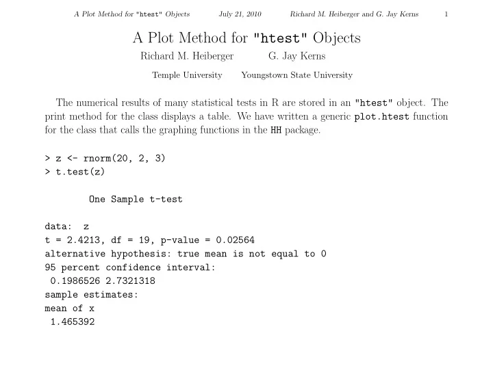
A Plot Method for "htest" Objects July 21, 2010 Richard M. Heiberger and G. Jay Kerns 1

A Plot Method for "htest" Objects

Richard M. Heiberger

• G. Jay Kerns

Temple University Youngstown State University

The numerical results of many statistical tests in R are stored in an "htest" object. The print method for the class displays a table. We have written a generic plot.htest function for the class that calls the graphing functions in the HH package. > z <- rnorm(20, 2, 3) > t.test(z) One Sample t-test data: z t = 2.4213, df = 19, p-value = 0.02564 alternative hypothesis: true mean is not equal to 0 95 percent confidence interval: 0.1986526 2.7321318 sample estimates: mean of x 1.465392

A Plot Method for "htest" Objects July 21, 2010 Richard M. Heiberger and G. Jay Kerns 2

> z <- rnorm(20, 2, 3) > t.test(z) One Sample t-test data: z t = 2.4213, df = 19, p-value = 0.02564 alternative hypothesis: true mean is not equal to 0 95 percent confidence interval: 0.1986526 2.7321318 sample estimates: mean of x 1.465392 > plot(t.test(z)) >

−1 1

t density: sx = 0.605, n =20, ν = 19

f(t) 0.0 0.1 0.2 0.3 0.4 0.5 0.6

−3 −2 −1 1 2 3

0.1 0.2 0.3 0.4 g( x ) = f(( x − µ i) s x) s x f(t) −2.093 2.093

t t

shaded area α = 0.0500

−1.267 1.267

x x

µ x

1.465

2.421

t

−2.421 p = 0.0256 One Sample t−test

A Plot Method for "htest" Objects July 21, 2010 Richard M. Heiberger and G. Jay Kerns 3

> vt <- var.test(x, y, alt="greater") > vt F test to compare two variances data: x and y F = 3.6, num df = 6, denom df = 18, p-value = 0.01598 alternative hypothesis: true ratio of variances is greater than 1 95 percent confidence interval: 1.35272 Inf sample estimates: ratio of variances 3.6 > plot(vt)

2 4 6 8 10

F density, ν1 = 6, ν2 = 18

F density

0.0 0.2 0.4 0.6 0.8

F 2.661

• crit. F

3.6

• bs. F

α = .050 p = .016

A Plot Method for "htest" Objects July 21, 2010 Richard M. Heiberger and G. Jay Kerns 4

We can specify the graph from the Rcmdr menu.

2 4 6 8 10

F density, ν1 = 6, ν2 = 18

F density

0.0 0.2 0.4 0.6 0.8

F 2.661

• crit. F

3.6

• bs. F

α = .050 p = .016

A Plot Method for "htest" Objects July 21, 2010 Richard M. Heiberger and G. Jay Kerns 5

RExcel Microsoft Excel is the most widely used spreadsheet program. Many of our clients and students use it as their data management system and as their working environment. On Windows RExcel and statconnDCOM (http://rcom.univie.ac.at) access COM— the Microsoft interprocess communications system, and seamlessly integrates the entire set of R’s statistical and graphical methods into Excel. Therefore these "htest" graphing methods are available through RExcel. The normal example is from the recent book R through Excel by Richard Heiberger and Erich Neuwirth. It is possible to build half the introductory course on this one graph. There are many more examples included with the software. There are several other talks at this UserR! 2010 conference illustrating applications of RExcel.

A Plot Method for "htest" Objects July 21, 2010 Richard M. Heiberger and G. Jay Kerns 6

−4 −2 2 4 6

Standard Normal Density N(0,1)

f(z) 0.0 0.1 0.2 0.3 0.4

−6 −5 −4 −3 −2 −1 1 2 3 4

0.1 0.2 0.3 0.4 g( x ) = f(( x − µ i) σ x) σ x f(z) −0.855

z1 z1

β = 0.1962 2.5 0.1 0.2 0.3 0.4 1.645

z z

shaded area α = 0.0500 µ

Placing values in the cells in Excel provides live control of the curve displayed in the R graph. The slider on µ1 in Excel, smoothly moves the normal curve centered at µ1 and adjusts the corresponding area illustrating β, the probability of the Type II Error.

A Plot Method for "htest" Objects July 21, 2010 Richard M. Heiberger and G. Jay Kerns 7

−4 −2 2 4 6

Standard Normal Density N(0,1)

f(z) 0.0 0.1 0.2 0.3 0.4

−7 −6 −5 −4 −3 −2 −1 1 2 3

0.1 0.2 0.3 0.4 g( x ) = f(( x − µ i) σ x) σ x f(z) −1.863

z1 z1

β = 0.0313 3.507 0.1 0.2 0.3 0.4 1.645

z z

shaded area α = 0.0500 µ

Placing values in the cells in Excel provides live control of the curve displayed in the R graph. The slider on µ1 in Excel, smoothly moves the normal curve centered at µ1 and adjusts the corresponding area illustrating β, the probability of the Type II Error.

A Plot Method for "htest" Objects July 21, 2010 Richard M. Heiberger and G. Jay Kerns 8

A Plot Method for "htest" Objects July 21, 2010 Richard M. Heiberger and G. Jay Kerns 9

2 4 6 8 10

F density, ν1 = 6, ν2 = 18

F density

0.0 0.2 0.4 0.6 0.8

Non−centrality parameter λ = 14 F 2.661

• crit. F

3.6

• bs. F

β = .352 1 − β = .648 α = .050 p = .016

A Plot Method for "htest" Objects July 21, 2010 Richard M. Heiberger and G. Jay Kerns 10

2 4 6 8 10

F density, ν1 = 6, ν2 = 18

F density

0.0 0.2 0.4 0.6 0.8

Non−centrality parameter λ = 14 F 2.661

• crit. F

3.6

• bs. F

α = .050 β = .352 1 − β = .648 p = .016

A Plot Method for "htest" Objects July 21, 2010 Richard M. Heiberger and G. Jay Kerns 11

2 4 6 8 10

F density, ν1 = 6, ν2 = 18

F density

0.0 0.2 0.4 0.6 0.8

Non−centrality parameter λ = 19 F 2.661

• crit. F

3.6

• bs. F

α = .050 β = .200 1 − β = .800 p = .016

A Plot Method for "htest" Objects July 21, 2010 Richard M. Heiberger and G. Jay Kerns 12

2 4 6 8 10

F density, ν1 = 6, ν2 = 18

F density

0.0 0.2 0.4 0.6 0.8

Non−centrality parameter λ = 14 F 2.661

• crit. F

3.6

• bs. F

β = .352 1 − β = .648 α = .050 p = .016

A Plot Method for "htest" Objects July 21, 2010 Richard M. Heiberger and G. Jay Kerns 13

2 4 6 8 10

F density, ν1 = 6, ν2 = 18

F density

0.0 0.2 0.4 0.6 0.8

Non−centrality parameter λ = 19 sx

2 = 7.2, sy 2 = 1

F 2.661

• crit. F

3.6

• bs. F

β = .200 1 − β = .800 α = .050 p = .016

A Plot Method for "htest" Objects July 21, 2010 Richard M. Heiberger and G. Jay Kerns 14

2 4 6 8 10

F density, ν1 = 6, ν2 = 18

F density

0.0 0.2 0.4 0.6 0.8

Non−centrality parameter λ = 19 F 2.661

• crit. F

3.6

• bs. F

α = .050 β = .200 1 − β = .800 p = .016

A Plot Method for "htest" Objects July 21, 2010 Richard M. Heiberger and G. Jay Kerns 15

Graphical Design

• 1. Color choice
• 2. Outline of p-value area
• 3. Alternate axes

In the normal and t plot, we show the ¯ x-scale, the z-scale under the null, and the z1-scale under the alternative. We can show the data scale for the F and χ2.

A Plot Method for "htest" Objects July 21, 2010 Richard M. Heiberger and G. Jay Kerns 16

Design Questions I invite discussion afterwards on these topics.

• 1. Color scheme
• 2. Legend vs Labels
• 3. Static vs Dynamic
• 4. Paper vs Screen

A Plot Method for "htest" Objects July 21, 2010 Richard M. Heiberger and G. Jay Kerns 17

Conclusions Dynamic graphs of hypothesis tests are an excellent way to understand the material and to teach the material. They can be used in production as part of experimental design. Inspecting these graphs can help in the determination of sample size.

A Plot Method for "htest" Objects July 21, 2010 Richard M. Heiberger and G. Jay Kerns 18

References

• 1. Baier, T. and Neuwirth, E. (2007) “Excel :: Com :: R”. Computational Statistics, 22 (1):

91–108. http://www.springerlink.com/content/uv6667814108258m/fulltext.pdf You can download this paper for no charge if your library subscribes.

• 2. Heiberger, Richard M., and Erich Neuwirth (2009). R through Excel: A Spreadsheet In-

terface for Statistics, Data Analysis, and Graphics, Springer–Verlag, New York. Series: Use R! http://www.springer.com/978-1-4419-0051-7

• 3. R Development Core Team (2010). R: A language and environment for statistical com-
• puting. R Foundation for Statistical Computing, Vienna, Austria. ISBN 3-900051-07-0,

http://www.R-project.org