SLIDE 1 A Panel Probit Model with Time-Varying Individual E¤ects
Jie Weia, Yonghui Zhangb
aSchool of Economics, Huazhong University of Science and Technology bSchool of Economics, Renmin University of China
November 7, 2019
Abstract This paper considers a probit model for panel data in which the individual e¤ects vary
- ver time by interacting with unobserved factors. In estimation we adopt a correlated ran-
dom e¤ects approach for individual e¤ects to get around the incidental parameter problem. This allows us to construct (asymptotically) unbiased estimators for average marginal ef- fects (AMEs), which are often the ultimate quantities of interest. We derive the asymptotic distributions for the AME estimators as well as provide the consistent estimators for their asymptotic variances. Next, we design a speci…cation test for detecting whether individual e¤ects are time-varying or not, and establish the asymptotic distribution for the proposed test statistic under the null hypothesis of no time variation of individual e¤ects. Monte Carlo simulations demonstrate satisfactory …nite sample performance of our proposed method. An empirical application to study the e¤ect of fertility on labor force participation (LFP) is
- provided. We …nd that fertility has a larger impact on female LFP in Germany than in the
US during the 1980s, and the e¤ect of fertility on LFP has turned even stronger in the 2010s in Germany, which calls for a reconsideration of relevant policies recently enacted such as the subsidized child care program. JEL Classi…cation: C23, C25 Key Words: Average marginal e¤ect, Correlated random e¤ect, Labor force participation, Minimum distance, Panel probit model, Time-varying individual e¤ect.
The authors are grateful to Iván Fernández-Val for providing his data and Matlab codes online and helpful
discussions, and to DIW Berlin for providing the German SOEP data. Wei gratefully acknowledges the …nancial support from the Ministry of Education of Humanities and Social Sciences Project of China (No.17YJC790159), the National Science Foundation of China (No.71803054), and Program for HUST Academic Frontier Youth
- Team. Zhang gratefully acknowledges the …nancial support from National Natural Science Foundation of China
(Projects No.71401166, No.71973141, and No.71873033). All errors are the authors’ sole responsibilities. Ad- dress correspondence to: Yonghui Zhang, School of Economics, Renmin University of China. E-mail address: yonghui.zhang@hotmail.com.
1
SLIDE 2 1 Introduction
Panel data models are widely used in empirical economics because they are capable of cap- turing the common feature among individuals, while allowing the possibility of controlling for unobserved individual heterogeneity, such as a …rm’s technology, consumer preference, and an employee’s latent ability. The individual heterogeneity is very likely to be correlated with regres- sors, and the failure to control for it would deliver inconsistent estimation and cause misleading statistical inference. While there are some well-established methods (e.g, within group or …rst di¤erence transfor- mation) to remove the unobserved individual heterogeneity in linear panel models, they usually fail in general nonlinear panels due to the nonlinear nature. Only for a few particular nonlinear models in which su¢cient statistics exist, can people obtain consistent estimation and valid in- ference results free from individual heterogeneity, such as Logit (see, e.g., Hsiao, 2014) and count data models (see, e.g., Hausman et al., 1984). To control for such heterogeneity in general, one usually has to treat individual e¤ects as nuisance parameters to be estimated (Fernández-Val, 2009). Unfortunately, this approach may still produce inconsistent estimators for parameters
- f interest if the number of time periods T is …xed. Even when T goes to in…nity at the same
rate as N, such estimators are still subject to asymptotic bias. So additional bias-reduction technique is needed for carrying out valid statistical inference, either by analytical or Jackknife correction; see Hahn and Newey (2004) and Fernández-Val (2009). However, these bias reduc- tion approaches typically involve intricate calculations or heavy computation for estimating or removing the bias terms. In contrast, as we will see later, the method proposed in our paper does not require any bias reduction. Furthermore, in the literature of nonlinear panel data models, the unobserved individual heterogeneity is usually treated as time-invariant. Obviously, such an assumption can be quite
- restrictive. As Bonhomme and Manresa (2016), this paper instead considers the time-varying
individual e¤ects (TVIE) in panel probit models, where the unobserved time-invariant individual …xed e¤ects are interactive with the unobserved time e¤ects as in Bai (2009). In practice, it is also more sensible to allow for the change of individual e¤ects across di¤erent time periods, for instance, when all individuals in economics are subject to period-speci…c common shocks. Our approach, compared with the usual one-way or two-way additive …xed e¤ects, permits the heterogeneous impacts of common shocks, and can include the usual …xed e¤ects speci…cations as special cases. In the literature of linear panel data models when T is small, TVIE has been investigated by Holtz-Eakin et al. (1988) and Ahn et al. (2001), among many others. Pesaran (2006), Bai (2009), and Moon and Weidner (2015) study TVIE in linear panel models when T is large. 2
SLIDE 3 In the nonlinear panel data models with interactive …xed e¤ects, Chen et al. (2019) study the estimation and inference assuming the number of factors is known; Boneva and Linton (2017) adopt the common correlated e¤ects approach (Pesaran, 2006) to estimate the panel binary choice model with a multi-factor error structure; Ando and Bai (2018) employ a Markov Chain Monte Carlo (MCMC) approach to deal with interactive …xed e¤ects in panel discrete choice
- models. All of these approaches require that both N and T go to in…nity jointly, whereas in our
setting only N goes to in…nity yet T is …xed, which is suitable for typical microeconomic panel data sets. Moreover, the knowledge of the true number of factors is not needed in this paper. Our approach to panel probit models hinges on a device of Mundlak-type Correlated Ran- dom E¤ects (CRE) together with a normality assumption on the projection errors. A similar approach to panel probit models with independently and identically distributed (IID) errors is also adopted by Wooldridge and Zhu (2019), who use the Lasso penalty to select variables in Chamberlain’s (1984) device with an additional sparsity assumption; Hsu and Shiu (2019) also employ the Mundlak-type CRE to control the correlation between regressors and …xed e¤ects in a semiparametric framework without using any distribution assumption on the projection errors. In this paper, with this Mundlak-type CRE device and distribution assumption, we can get rid
- f the nuisance parameters by integrating them out and then obtain consistent estimators for
parameters of our interest. Note that the original sets of parameters cannot be identi…ed without further restrictions under our TVIE assumption and heteroskedastic errors. However, we can still recover and derive asymptotically unbiased estimators for Average Marginal E¤ects (AMEs) which are often the ultimate quantities of interest (see, e.g., Angrist (2001) and Wooldridge (2010)). More importantly, there is no additional bias reduction for our approach. For the purpose of inference with AMEs, we establish the asymptotic distribution and provide a consistent estimator for its variance under some mild conditions. Furthermore, by this approach one can conduct estimation and inference for period-speci…c AMEs, and thus capture the dynamics of AMEs. Note that the ignorance of time variation in individual e¤ects may result in substantial bias for the AME estimator, and thus render the subsequent inference misleading. Concerned about the consequence, we further propose a test to check whether individual e¤ects are time-invariant
- r not, allowing for either homoskedastic or heteroskedastic error terms. The speci…cation test
- f TVIE is also considered by Bai (2009), yet his test is only applicable to linear panel models.
Our proposed test is inspired by the Minimum Distance (MD) estimator in Chamberlain (1982). We impose the nonlinear restrictions of time-invariant individual e¤ects in the MD estimation, and the eventual test statistic follows as the minimized distance. We show that under some regular conditions the test statistic follows a Chi-squared distribution asymptotically under the 3
SLIDE 4 null hypothesis of no time variation of individual e¤ects. The Monte Carlo simulation evidence highlights both accuracy and robustness of our pro- posed estimators for AMEs at …nite samples, in comparing with several existing main methods for panel probit models. The …nite sample performance of our proposed speci…cation test is also satisfactory in simulations. In an empirical application, we apply our method to study how labor force participation (LFP) of married women depends on fertility in the US and Germany. We …nd signi…cant di¤erences for the speci…cation of individual e¤ects as well as the AMEs
- f fertility across the two countries in the 1980s. A further study on the German job market
in the 2010s reveals even a stronger negative e¤ect of fertility on LFP, suggesting limitation and ine¤ectiveness of recently enacted policies in Germany, such as the subsidized child care program. The rest of the paper is organized as follows. In Section 2, we introduce the model, propose
- ur estimators for AME and study their large sample property. In Section 3, we construct a
speci…cation test for the presence of time-varying individual e¤ects. Monte Carlo results and an empirical illustration are given in Sections 4 and 5, respectively. Section 6 concludes. The proofs of main results are relegated to the Appendix.
2 The TVIE Panel Probit Model and the Estimators
A binary choice panel data model with time-varying individual e¤ects can be written as Yit = 1
it + 0 ift + uit > 0
i = 1; : : : ; N; t = 1; : : : ; T; (2.1) where Yit is a binary response variable, 1() is the usual indicator function, Xit is a p 1 vector
- f regressors, denotes a p 1 vector of parameters (index coe¢cients), ft is a R 1 vector of
unobserved time e¤ects or factors, i is a R 1 vector of unobserved individual …xed e¤ects or factor loadings, and uit is the idiosyncratic error. As the classical …xed e¤ects, both ft and i are possibly correlated with Xit. When ft is a constant vector for all t’s, model (2.1) reduces to the usual panel binary choice model with time-invariant individual …xed e¤ects. In this paper, we allow for arbitrary heteroskedasticity and serial correlation of uit along time such that ui (ui1; ; uiT )0 IID N(0; u), where u is a T T covariance matrix with the (t; s)th element being ts. We are interested in estimating the average marginal e¤ects (AMEs) when N is large and T is …xed. Since ft’s are of …nite dimensions and repeatedly measured for N times, we treat them as unknown parameters. As the individual …xed e¤ect i is typically correlated with Xit, to purge this endogeneity problem, we follow Mundlak (1978) and adopt the CRE for i as an auxiliary regression i = 0 + Xi + i; (2.2) 4
SLIDE 5 where Xi T 1 PT
t=1 Xit, 0 is a (R 1) vector of constants, is a (R p) matrix of unknown
coe¢cients, and i is the vector of associated linear projection errors (R 1) with E(i) = 0 and is independent of fXit; uitgT
t=1. The Mundlak-type CRE is widely used in the literature of
panel data models; see Wooldridge (2010). Recently, both Hsu and Shiu (2019) and Wooldridge and Zhu (2019) adopt some similar devices to model the relationship between individual …xed e¤ects and regressors. Note that Chamberlain’s (1982) general CRE can be written as i = 0 + PT
t=1 tXit + i, where t is a period-speci…c unknown matrix of coe¢cients. Then our
Mundlak device in (2.2) can be seen as a restricted version of Chamberlain’s CRE. However, our approach can preserve parsimony and avoid the “time inconsistency” problem of Chamberlain’s general CRE in modelling the relationship between i and Xit’s. With these imposed conditions, it comes to that Yit = 1(X0
it + 0 0ft +
X0
i0ft + "it > 0);
(2.3) where the composite error "it f0
ti + uit includes two components: the …rst term (f0 ti) comes
from the linear projection error in (2.2) and the second term (uit) is the original idiosyncratic error in (2.1). Let !t Var("it) = 2
t + f0 tft, where 2 t is the tth diagonal element of u and
=Var(i). Clearly, both time-variation in individual e¤ects and the heteroskedasticity of uit are the sources of the heteroskedasticity of "it. De…ne 0t 0
0ft
p!t , t
, t 0ft p!t , and "
it "it
p!t : (2.4) Clearly, the heteroskedasticity of "it leads to the time heterogeneity of parameters. With (2.4),
- ur model can be written as
Yit = 1(0t + X0
itt +
X0
it + " it > 0);
where Var("
it) = 1:1 Note that given ft the distribution of " it is still unknown without specifying
the distribution of i. Following Wooldridge and Zhu (2019), we impose a strong assumption
- n the distribution of the projection error i. Speci…cally, we assume that i is independent of
fXit; uitgT
t=1 and i IID N(0; ). Then it follows that
"
i = (" i1; ; " iT )0 IID N(0T1; ")
where ";ts = ts+f0
sft
p!t!s
is the (t; s)th element of " and the diagonal element is ";tt = 1. The full information maximum likelihood estimation (FMLE) with identi…cation conditions on , via a T-dimensional integration of a multivariate normal probability density function, should
1Since and !t are nonseparable, some possible identi…cation conditions such as the …rst element of being
1 or kk = 1 can be applied to identify , where kk is the Euclidean norm, if one is interested in this parameter.
5
SLIDE 6 be e¢cient for the estimation of from the classical MLE theory. However, it is quite expensive to do so either by the numerical approximation or some simulation methods due to the nonlinear nature of the model. Instead, in this paper, we consider the simple estimation of (0t; t,t) by the standard probit regression method based on the observations at the tth period. De…nitely,
- ur approach would su¤er some e¢ciency loss in the estimation of without using the fact that
all t’s can be written as t = p!t, but can avoid large dimensional numerical integration and greatly reduce the computation burden, particularly when T is not very small. In addition, our approach enables researchers to estimate period-speci…c AMEs which not only rely on but also on some other period-speci…c parameters such as ft and !t. Lastly, our period-by-period estimator can capture the dynamic of AMEs and is also particularly suitable for constructing the speci…cation test for the time-invariance of individual e¤ects, as will be seen in the next section. Under the usual strict exogeneity assumption for static models,2 the moment condition for the tth period is Pr(Yit = 1jXit; Xi) = (0t + X0
itt +
X0
it);
(2.5) where () is the cumulative distribution function (CDF) of N(0; 1). Clearly, (2.5) demonstrates the success in removing unobserved individual heterogeneity, and Xi here plays a similar role
- f su¢cient statistic for i, just as in panel Poisson regression for count data. We denote the
estimators in cross-sectional probit regression of the tth time period as ^ 0t, ^ t, and ^
argued before, is not identi…ed without further restrictions on it. Fortunately, from the results
- f period-speci…c probit regression, we are able to obtain adequate information to recover the
period-speci…c summary measures, which can provide consistent estimates of casual e¤ects and are often the ultimate quantities of interest to researchers. In this paper, we are interested in the estimation of AME for each period and the average AME across time periods. As for the vector of AMEs at each period, it refers to averaging the individual marginal e¤ects across the population at a given time t, which is given by t
@Xit E(YitjXit; i)
= E
@Xit
it + 0 ift
pt
= E
@Xit
it + 0 ift
pt
Xi
= tE
itt +
X0
it)
(2.9)
2As a matter of fact, we only need that uit is independent of Xit and
Xi, which is slightly weaker than the assumption of strict exogeneity of Xit’s.
6
SLIDE 7 where the last expectation in (2.9) is taken with respect to Xit and Xi jointly. The de…nition of AME in (2.6) originates from Chamberlain (1984) and is also adopted by Fernández-Val (2009)
- recently. Sometimes, one may be more interested in the time average of AMEs:
- T 1
T
T
X
t=1
t = 1 T
T
X
t=1
tE
itt +
X0
it)
(2.10) Then the parameters of interest t, = (0
1; ; 0 T )0 ; and
T can be respectively estimated by b t = 1 N
N
X
i=1
^ t(^ 0t + X0
it^
t + X0
i^
t); (2.11) b
1; ; b T
0 ; and (2.12) b
= 1 NT
T
X
t=1 N
X
i=1
^ t(^ 0t + X0
it^
t + X0
i^
t): (2.13) Before proceeding, we de…ne some notations. Let Wit
it;
X0
i
0 and t
t; 0 t
0. Denote qit 2Yit 1, ait (t)
qit(qitW 0
itt)
(qitW 0
itt) , and HN;t (t)
1 N
PN
i=1 ait (ait + W 0 itt) WitW 0 it,
where ait = ait (t). Let 0
t denote the true value of t; a0 it = ait
0 =
1 ; ; 00 T
- 0. We denote the true values for t, , and
T by 0
t , 0, and T , respectively.
To establish the asymptotic distribution of b , we make the following assumptions. Assumption 1. (i) ui (ui1; ; uiT )0 IID N(0; u), and uit are independent of Xjs and fs for all i; j; t, and s; (ii) Xi’s are identically distributed and conditional independent across i given F (f1; ; fT ) and max1tT E kXitk4 < 1; (iii) i, the linear projection error of i on Xi; follows IID N(0; ), and is independent of Xjs, ujs and fs all i; j;and s; (iv) For each t = 1; : : : ; T, 0
t lies in the interior of t, where t is a compact subset of R1+2p;
(v) Ht plimN!1 HN;t
- t
- exists and is nonsingular for t = 1; : : : ; T.
Remark 1. Assumption 1(i) speci…es the joint normality distribution of the errors and allows for heteroskedasticity and serial correlation of uit’s along time; 1(ii) assumes cross-sectionally conditional independence of Xi given F, where we see ft’s as random variables although they are treated as unknown parameters; 1(ii) can be easily relaxed to allow for heterogenous distribution
- f Xi across i; 1(iii) further makes a strong distribution assumption (the normality) on the linear
projection i, which is used to integrate out the unobserved individual heterogeneity; also see Wooldridge and Zhu (2019). Assumptions 1(iv)-(v) are both standard conditions used in the likelihood approach to nonlinear panel data models with …xed T. 7
SLIDE 8 Let ^ (^
- 1; ; ^
- T )0 denote the estimator of (0
1; ; 0 T )0. Let 'it H1 t
Wita0
it and
'i = ('0
i1; ; '0 iT )0. De…ne i;ts Cov('it; 'is) = H1 t
E
isa0 ita0 is
s
be the dp dp covariance matrix, where dp (1+2p). We …rst state a proposition on the limiting distribution of ^ , which is used to establish the asymptotic properties of b t, b ; and b
- T as well as the speci…cation
test in the next section. Proposition 2.1 Under Assumption 1, we have as N ! 1, p N
0 d ! N(0; ); where B B @ 11 1T . . . ... . . . T1 TT 1 C C A is a Tdp Tdp matrix and ts = limN!1 1
N
PN
i=1 i;ts.
Remark 2. (i) The proof of the above proposition is standard since we estimate ^ t’s by the period-by-period cross-sectional probit regression. When T is …xed, it is straightforward to establish the joint limiting distribution of ^ by the Cramér-Wold device. A proof sketch is provided in the Appendix. (ii) Proposition 2.1 implies that: (a) ^ is an asymptotically unbiased estimator for , and (b) ^ t and ^ s are jointly asymptotically normally distributed with asymptotic covariance ts for t 6= s. Remark 3. If is the parameter of interest, we can estimate by a linear combination of ^ t’s, i.e., ^ = T 1 PT
t=1 ct^
t; where ct is the adjustment coe¢cient for the tth period estimator ^ t: For example, ct =
t
when the identi…cation restriction kk = 1 is imposed, and ct = ^ t=[^ t;11(^ t;1 6= 0)] when the …rst element of is …xed at one. It is straightforward to establish the large sample theory for the estimator ^ based on Proposition 2.1. The results are
- mitted since we focus on the estimation of AMEs in this paper.
Before stating the asymptotic distribution of b , we further give some notations. Denote a Tp 1 vector i () = (i1(1)0; ; iT (T )0)0 where it(t) t(W 0
itt). Let it = it(0 t ),
D0
t E
t )
@0
t
Let D0 Diag
1; ; D0 T
- be a Tp Tdp blockwise diagonal matrix.
Denote B B @ 11 1T . . . ... . . . T1 TT 1 C C A with ts =Cov(it; is). Theorem 2.2 Under Assumption 1, as N ! 1, we have p N
0 d ! N(0; ); (2.14) where = +D0D00 = B B @ 11 + D0
111D00 1
1T + D0
11T D00 T
. . . ... . . . T1 + D0
T T1D00 1
TT + D0
T TT D00 T
1 C C A is a TpTp matrix. 8
SLIDE 9 Remark 4. (i) The above theorem establishes the joint limiting distribution of b = (b 1; ; b T ) as N ! 1. Using Proposition 2.1, we can prove the theorem with the Taylor expansion and the central limit theorem (CLT) for independent but not identically distributed random variables. The proofs are relegated to the Appendix. (ii) Theorem 2.2 shows that our AME estimator is asymptotically unbiased and therefore there is no need to do bias correction. (iii) Based on Theorem 2.2, one can easily construct tests for the equality of two period-speci…c AMEs such as 0
t = 0 s or 0 t;l = 0 s;l for the lth variables (1 l p) for t 6= s.
From Theorem 2.2, we can easily obtain the asymptotic distributions of b t for each t = 1; : : : ; T and b
- T , which are given in the following corollary.
Corollary 2.3 Under Assumption 1, as N ! 1, we have for t = 1; : : : ; T p N
t 0
t
d ! N(0; tt); (2.15) where tt = tt + D0
t ttD00 t , and
p N b
T
d ! N(0; 0
T );
(2.16) where 0
T T 2 PT t=1
PT
s=1
t tsD00 s
The proofs for the corollary are straightforward by the continuous mapping theorem (CMT). For the purpose of inference about AMEs t and T , we need to provide consistent estimators for tt and 0
T . To this end, de…ne
^ ts = 1 N
N
X
i=1
it(^ t)is(^ s)0 " 1 N
N
X
i=1
it(^ t) # " 1 N
N
X
i=1
is(^ s)0 # , (2.17) ^ D0
t
= 1 N
N
X
i=1
@it(^ t) @0
t
; and ^ ts = 1 N
N
X
i=1
^ 'it^ '0
is;
(2.18) for t; s = 1; : : : ; T, where ^ 'it = H1
N;t(^
t)Witait(^ t). Then the estimators for variance matrices tt and 0
T are respectively given by
^ tt = ^ tt + ^ D0
t ^
tt ^ D00
t and ^ T = 1
T 2
T
X
t=1 T
X
s=1
ts + ^ D0
t ^
ts ^ D00
s
(2.19) The following proposition provides the consistency of ^ tt and ^
T .
Proposition 2.4 Under Assumption 1, as N ! 1, we have (i) ^ tt = tt + op (1) for t = 1; : : : ; T, and (ii) ^
T = 0 T + op (1).
Remark 5. Based on Theorem 2.2 and Proposition 2.4, we can carry out valid inference on the period-speci…c AMEs t and the time average of AMEs T . A sketch proof for the above proposition is given in the Appendix. Also note that no knowledge about the true number of factors R is needed in estimation or inference on AMEs. 9
SLIDE 10 3 A Speci…cation Test of TVIE
Ignoring the time variation of individual e¤ects may render considerable bias of the AME esti- mator, and hence invalidate inference. Such a consequence is demonstrated in our Monte Carlo simulations in the next section. To guard against misspeci…cation of the individual e¤ects, here we formally develop a test to detect the time variation of individual e¤ects due to the presence
The null hypothesis of time invariant individual e¤ects can be written as H0 : ft = f(0) for some f(0) 6= 0 and t = 1; : : : ; T, (3.1) and the alternative hypothesis is H1 : ft 6= fs for some t 6= s and t; s = 1; : : : ; T: (3.2) The basic idea for our test is straightforward. Our previously obtained estimator ^ from sequential estimation is consistent under both H0 and H1. We can also estimate under the restrictions from H0, and denote the estimator as ~ . Clearly, the estimator ~ is consistent only when H0 is true. Such di¤erent behaviors of ^ and ~ motivate us to construct a test statistic by comparing these two estimators. Recall that t = (0
t; 0t; 0 t)0 with 0t = 0 0ft=!1=2 t
; t = =!1=2
t
; and t = 0ft=!1=2
t
: For reference hereafter, denote the counterpart of t with restrictions under H0 as y
t = (y0 0t; y0 t ; y0 t )0,
where y0
0t = 0 0f(0)=!1=2 t
, y
t = =!1=2 t
; and y
t = 0f(0)=!1=2 t
: Although t and y
t are both time-varying, y t is expected to ful…ll the additional requirement
that y
t=y 0t = =0 0f(0) and y t=y 0t = 0f(0)=0 0f(0)
are both time-invariant, whereas t is not subject to these constraints since t=0t = =0
0ft
and t=0t = 0ft=0
0ft are both time-varying in general.
In order to estimate the restricted parameter y
t, one possibility is to employ full information
- MLE. Once again, the computation burden might be overwhelming even for moderately large T.
An easier alternative is to construct the minimum distance estimator in the spirit of Chamberlain (1982). To describe the method, let # = (y
01; ; y 0T ; Cy0 1 ; Cy0 2 )0 2 , where Cy 1 = =0 0f(0) and
Cy
2 = 0f(0)=0 0f(0), and RT+2p. Under H0, the parameter y
1 ; ; y0 T
depends on # through a function, which we shall denote by G(), such that y = G(#) = (y
01; ; y 0T )0 (1; Cy0 1 ; Cy0 2 )0:
10
SLIDE 11 We write the estimation problem with imposed restrictions by solving the minimum distance (MD) estimator as follows. min
#2
h ^ G(#) i0 ^ 1 h ^ G(#) i ; (3.3) where ^ 1 is the weight matrix with ^ being a consistent estimator of given in Proposition 2.1. See (2.18) for our proposed estimator ^ ts, which is the (t; s)th block of ^ . Denote the solution to the minimization problem in (3.3) by ~ #. We then propose the following test statistic J = N h ^ G(~ #) i0 ^ 1 h ^ G(~ #) i : (3.4) Theorem 3.1 Suppose that is a compact subset of RT+2p and 0
0f(0) 6= 0 under H0. Under
Assumption 1, as N ! 1, we have J
d
! 2
2(T1)p;
when H0 holds. Remark 6. Theorem 3.1 provides the asymptotic pivotal distribution of our test statistic with large N and …xed T under H0. It is easy to implement our test in practice. Also noting that under the …xed alternative H1, the MD estimator is inconsistent in general. Hence J diverges to in…nity with the rate of Op (N), so as to produce the power of the test. Remark 7. If H0 in (3.1) cannot be rejected, we can further design a test for the presence
- f heteroskedasticity of the errors.
When there is no heteroskedasticity, i.e., Var(uit) = 2 for all t’s, we have t = (0) for some constant vector (0) since !t = 2 + f(0)0f(0) for all t’s. The homogeneity restriction of parameters across t can be used to construct a test for the heteroskedasticity of uit in the same spirit as J in (3.4).
4 Monte Carlo Simulations
In simulations, we design the following data generating processes (DGPs): Yit = 1
ift + uit > 0
where 0 = 1 and other components are generated as follows: (i) The scalar regressor Xit follows an AR(1) process and has time-varying …xed e¤ects: Xit = 0:5Xi;t1 + 0:50
Rft + eit; where
eit IID N (0; 1) and R is the R 1 vector of ones. We set Xi0 = 0 as the initial value. (ii) Both time-varying and time-invariant individual e¤ects are considered: 11
SLIDE 12
- 1. Time-varying case: (a) The individual …xed e¤ects i’s are generated according to
the Mundlak-device: i = 0 + Xi + i; where Xi = T 1 PT
t=1 Xit and i IID
N (0; IR) : We set 0 = R and = R. (b) The time-varying factors ft’s are gen- erated according to stationary AR(1) processes: ft = 0:5ft1 + vt; where vt IID N
- 0; R1IR
- : Let f0 = 0R1 be the initial values of the factor processes.
- 2. Time-invariant case: (a) The individual …xed e¤ects i’s are scalars and generated
according to the Mundlak-device: i = 1 + Xi + i; where i IID N (0; 1) : (b) The factor ft is …xed at 0.5 for all t’s. Then the individual e¤ects are given by ift = 0:5i for i = 1; : : : ; N: (iii) The error term uit follows an AR(1) process: uit = 0:5ui;t1 + &it, where ui0 = 0 and &i (&i1; ; &iT )0 IID N (0; &). We set & =Diag(&;11; ; &;TT ) with &;tt = 0:25
i=1 Xit
We examine the …nite sample performance of our proposed estimators for AMEs and spec- i…cation test for time-varying individual e¤ects. In simulations, di¤erent sample sizes N = 200; 400; 800, and T = 3; 6 are under investigation. For each combination of sample sizes, the number of replications is 1000 for both estimation and testing. Tables 1 and 2 report the ratio of various (time average) AME estimators to the true value (
T ) when T is 3 and 6, respectively.3 We compare our estimator (TVIE) with other estimators
mainly used in panel probit models. Let HN-A and HN-M be the one-step analytical bias- corrected estimators of Hahn and Newey (2004) based on the maximum likelihood approach and the general estimating equations, respectively, denote HN-JK as the Hahn and Newey’s (2004) bias-corrected estimator based on the leave-one-period-out jackknife, and let FVBC be the Fernández-Val’s (2009) bias-corrected estimator. The performance of estimators are evaluated by various criteria as in Fernández-Val (2009). Based on the ratio of AME estimators to
T ,
we report the mean, median, SD (the standard deviation), SE/SD (the ratio of the average standard error to SD), and MAE (median absolute error) for the estimators.4 As in Hahn and Newey (2004) and Fernández-Val (2009), “p;.05” and “p;.10” stand for rejection frequencies with nominal values 0.05 and 0.10, respectively. The results exhibit superior …nite sample performance of our AME estimators, whereas the alternative estimators su¤er from relatively large bias. FVBC is the least biased among the four alternative estimators. However, it is subject to substantial over-rejection in testing, mainly due
3Recall that T is de…ned in (2.10) when = 0. 4We report MAE instead of root mean squared error (RMSE) by following Fernández-Val (2009), because the
MLE estimators might be explosive in …nite samples.
12
SLIDE 13 Table 1: Estimation results of
T when T = 3
N Estimator Mean Median SD p; .05 p; .10 SE/SD MAE Panel A: R = 1 200 TVIE 1.001 0.999 0.138 0.063 0.123 0.878 0.083 HN-A
0.892 277.804 0.665 0.716 0.000 0.262 HN-M 1.144 1.106 0.371 0.583 0.635 0.217 0.190 HN-JK 1.580 1.502 0.510 0.871 0.901 0.174 0.503 FVBC 1.015 0.965 0.316 0.518 0.582 0.263 0.162 400 TVIE 0.998 0.996 0.094 0.052 0.105 0.923 0.057 HN-A 0.880 0.908 0.515 0.728 0.767 0.122 0.245 HN-M 1.076 1.037 0.326 0.635 0.686 0.179 0.164 HN-JK 1.578 1.494 0.469 0.937 0.950 0.131 0.495 FVBC 1.017 0.952 0.300 0.623 0.677 0.196 0.150 800 TVIE 0.998 0.998 0.065 0.058 0.111 0.921 0.037 HN-A 0.918 0.916 0.643 0.818 0.850 0.068 0.223 HN-M 1.025 0.976 0.327 0.719 0.769 0.127 0.153 HN-JK 1.585 1.456 0.493 0.961 0.967 0.087 0.456 FVBC 1.021 0.936 0.307 0.742 0.789 0.134 0.154 Panel B: R = 2 200 TVIE 1.010 1.001 0.148 0.055 0.116 0.876 0.085 HN-A
0.938 51.952 0.608 0.669 0.002 0.241 HN-M 1.209 1.157 0.393 0.580 0.631 0.224 0.214 HN-JK 1.664 1.532 0.748 0.868 0.891 0.128 0.535 FVBC 1.082 1.003 0.450 0.473 0.541 0.202 0.152 400 TVIE 1.015 1.005 0.135 0.070 0.123 0.690 0.060 HN-A 0.875 0.951 1.130 0.668 0.728 0.060 0.193 HN-M 1.144 1.095 0.317 0.606 0.657 0.196 0.169 HN-JK 1.622 1.507 0.557 0.936 0.952 0.120 0.508 FVBC 1.058 0.979 0.337 0.553 0.616 0.190 0.136 800 TVIE 1.000 0.996 0.080 0.066 0.114 0.789 0.041 HN-A 0.987 0.980 0.487 0.746 0.792 0.095 0.184 HN-M 1.083 1.050 0.310 0.687 0.731 0.137 0.146 HN-JK 1.612 1.488 0.500 0.968 0.974 0.092 0.489 FVBC 1.052 0.974 0.298 0.677 0.716 0.147 0.131 Note: The results are based on the ratio of estimators to the true value (b
T ).
13
SLIDE 14 Table 2: Estimation results of
T when T = 6
N Estimator Mean Median SD p; .05 p; .10 SE/SD MAE Panel A: R = 1 200 TVIE 0.995 0.994 0.075 0.054 0.107 0.931 0.045 HN-A 1.281 1.229 0.346 0.790 0.821 0.163 0.244 HN-M 1.275 1.212 0.362 0.767 0.810 0.155 0.214 HN-JK 1.288 1.204 0.456 0.758 0.796 0.127 0.214 FVBC 1.209 1.154 0.336 0.682 0.730 0.169 0.168 400 TVIE 0.995 0.994 0.054 0.048 0.098 0.931 0.035 HN-A 1.167 1.247 3.393 0.864 0.884 0.012 0.257 HN-M 1.270 1.218 0.305 0.830 0.865 0.130 0.233 HN-JK 1.291 1.215 0.371 0.835 0.865 0.111 0.229 FVBC 1.212 1.165 0.302 0.752 0.779 0.133 0.184 800 TVIE 0.994 0.992 0.041 0.056 0.106 0.877 0.024 HN-A 1.281 1.238 0.307 0.891 0.902 0.093 0.247 HN-M 1.268 1.212 0.313 0.892 0.912 0.091 0.222 HN-JK 1.300 1.221 0.398 0.906 0.923 0.074 0.231 FVBC 1.204 1.158 0.293 0.802 0.829 0.098 0.180 Panel B: R = 2 200 TVIE 0.997 0.997 0.082 0.051 0.106 0.912 0.050 HN-A 1.321 1.269 0.407 0.799 0.830 0.149 0.277 HN-M 1.323 1.254 0.369 0.784 0.822 0.164 0.259 HN-JK 1.335 1.248 0.417 0.763 0.799 0.150 0.255 FVBC 1.262 1.193 0.356 0.702 0.746 0.171 0.208 400 TVIE 1.001 0.998 0.061 0.059 0.115 0.874 0.035 HN-A 1.338 1.284 0.383 0.896 0.908 0.112 0.291 HN-M 1.346 1.256 0.464 0.873 0.894 0.092 0.260 HN-JK 1.373 1.252 0.560 0.881 0.905 0.079 0.263 FVBC 1.282 1.201 0.417 0.798 0.827 0.104 0.209 800 TVIE 1.000 0.995 0.052 0.070 0.135 0.724 0.026 HN-A 1.337 1.263 0.356 0.913 0.932 0.086 0.273 HN-M 1.331 1.237 0.488 0.892 0.912 0.062 0.240 HN-JK 1.365 1.237 0.577 0.902 0.914 0.054 0.243 FVBC 1.264 1.181 0.432 0.827 0.844 0.071 0.193 14
SLIDE 15 to the underestimation of dispersion, apparent in the values of SE/SD. Our estimator TVIE has a relatively small bias and much more accurate estimation for the dispersion, so that its rejection frequencies are much closer to the nominal levels. It suggests that the asymptotic distribution that we have derived can approximate the …nite sample distribution reasonably well. For the sake of robustness, we also do experiments with usual time-invariant individual e¤ects, i.e., the case with R = 0. Table 3 compares our method and alternatives when T = 3 and 6. It is clear that our proposed TVIE estimator is quite robust under this setting. More interestingly, the TVIE still outperforms the alternatives, especially when T is small (T = 3). The under performance of the alternatives is probably due to the ignorance of heteroskedasticity, whereas our approach allows and accounts for heteroskedasticity by adapting our estimators to
- it. As T gets bigger, the four alternative methods get more accurate in terms of estimation bias,
which comes closer to the bias of TVIE, yet they still su¤er from remarkable underestimation of dispersion, yielding considerably higher rejection frequencies than their corresponding nominal levels. Next, we examine the …nite sample performance of our speci…cation test for TVIE. The null hypothesis of time-invariant individual e¤ects corresponds to the case with R = 0, while the alternative hypotheses of TVIE are …xed at R = 1 and R = 2, respectively. Table 4 reports rejection frequencies under the null (size) and two alternatives (power), at nominal values of 10%, 5%, and 1%, respectively. The results show that our test controls the size reasonably well although there is a little bit of size distortion (undersize) when T = 6 and N = 400 and 800, and it has power approaching one at a moderate sample size.
5 An Empirical Application
In this section, we apply our method to study the e¤ect of fertility on labor force participation (LFP), which has attracted a lot of attention in labor economics; see, e.g., Hotz and Miller (1988), Angrist and Evans (1998), Carrasco (2001), Francesconi (2002), Attanasio et al. (2008), Daniela and Robert (2009), and Hwang et al. (2018). The study is perhaps more relevant and valuable now than ever as many developed countries are su¤ering from the problems of slow economic growth and rapid aging. As pointed out by Angrist and Evans (1998) and Carrasco (2001), fertility and LFP are most likely jointly determined. A panel data model is expected to mitigate the self-selection bias as it takes into account of unobserved heterogeneity, which is further allowed to be time-varying in our setup. The purpose of the empirical application is twofold. First, it illustrates the usage of our proposed method and provides a comparison between the US and German job markets in the 15
SLIDE 16 Table 3: Estimation results of
T when R = 0
N Estimator Mean Median SD p; .05 p; .10 SE/SD MAE Panel A: T = 3 200 TVIE 0.994 0.992 0.113 0.056 0.117 0.962 0.076 HN-A 0.410 0.569 0.632 0.873 0.901 0.120 0.431 HN-M 0.933 0.925 0.143 0.414 0.500 0.484 0.122 HN-JK 1.283 1.279 0.188 0.769 0.808 0.377 0.279 FVBC 0.802 0.803 0.094 0.727 0.794 0.738 0.197 400 TVIE 0.997 0.997 0.078 0.042 0.106 0.988 0.055 HN-A 0.547 0.640 0.347 0.941 0.955 0.158 0.360 HN-M 0.898 0.880 0.104 0.591 0.664 0.479 0.126 HN-JK 1.289 1.283 0.127 0.946 0.952 0.383 0.283 FVBC 0.805 0.804 0.062 0.926 0.954 0.784 0.196 800 TVIE 0.994 0.996 0.054 0.049 0.106 1.001 0.038 HN-A 0.621 0.673 0.230 0.984 0.989 0.168 0.327 HN-M 0.864 0.853 0.067 0.846 0.881 0.543 0.147 HN-JK 1.292 1.291 0.092 0.993 0.995 0.371 0.291 FVBC 0.807 0.807 0.045 0.969 0.970 0.770 0.193 Panel B: T=6 200 TVIE 0.997 0.996 0.068 0.060 0.104 0.984 0.043 HN-A 0.985 0.990 0.126 0.235 0.312 0.398 0.054 HN-M 1.011 1.009 0.078 0.200 0.289 0.646 0.053 HN-JK 1.027 1.023 0.088 0.242 0.323 0.581 0.056 FVBC 0.951 0.950 0.070 0.264 0.361 0.719 0.061 400 TVIE 0.996 0.995 0.047 0.049 0.099 0.998 0.033 HN-A 0.990 0.988 0.061 0.240 0.321 0.585 0.039 HN-M 1.010 1.009 0.056 0.226 0.313 0.631 0.039 HN-JK 1.030 1.029 0.062 0.292 0.376 0.574 0.045 FVBC 0.953 0.952 0.050 0.335 0.441 0.716 0.051 800 TVIE 0.995 0.994 0.034 0.065 0.120 0.980 0.024 HN-A 0.986 0.992 0.113 0.263 0.339 0.222 0.029 HN-M 1.009 1.010 0.042 0.268 0.345 0.596 0.029 HN-JK 1.029 1.025 0.054 0.318 0.398 0.465 0.034 FVBC 0.951 0.949 0.036 0.502 0.591 0.700 0.051 16
SLIDE 17 Table 4: Empirical rejection frequencies of the test for time invariance of individual e¤ects size (R=0) power (R=1) power (R=2) T N 10% 5% 1% 10% 5% 1% 10% 5% 1% 3 200 0.092 0.048 0.018 0.894 0.868 0.821 0.867 0.846 0.791 400 0.104 0.065 0.025 0.928 0.916 0.885 0.923 0.904 0.866 800 0.088 0.040 0.008 0.964 0.953 0.935 0.928 0.918 0.896 6 200 0.101 0.060 0.031 0.994 0.989 0.978 0.993 0.989 0.984 400 0.070 0.050 0.024 0.999 0.996 0.993 0.994 0.992 0.986 800 0.048 0.029 0.014 1.000 0.998 0.997 0.998 0.998 0.993 1980s. Second, it draws some new conclusions on the causal e¤ect of fertility on LFP and sheds light on the e¤ect of recently enacted policies, such as subsidized child care programs, by providing evidence based on the German job market in the 2010s.
5.1 The e¤ects of fertility on LFP in the US and Germany in the 1980s
We …rst use the same data set from the Panel Study of Income Dynamics (PSID) as Fernández- Val (2009), which can be downloaded from http://sites.bu.edu/ivanf/research/. The sample contains yearly observations for the 9 calendar years 1980-1988. 1200 women in the US aged 22-45 in 1980, who were continuously married with husbands in the labor force in each period, are included in the sample,5 and 556 of them changed LFP status during the sample
- period. The explanatory variables, which are taken as the same with Fernández-Val (2009),
include numbers of children from three groups: 0-2, 3-5, and 6-17 year-olds. Also included are the logarithm of husbands (real) income, age and square of age. The dependent variable is the female LFP (1 for working while 0 for non-working). The descriptive statistics for the PSID sample are listed in Panel A of Table 5. The second data set in use is from German Socio-Economic Panel (SOEP), which we obtain from the DIW, Berlin; see https://www.diw.de/en/soep. For the sake of comparison, we would choose a sample during the same time span (1980-1988) as the PSID sample. However, the SOEP data prior to 1984 are not available, so we end up with a sample for the 5 years 1984-
- 1988. 1528 women are included by the same criteria as in the PSID data. We keep using the
same set of explanatory variables with a subtle di¤erence: since SOEP has no speci…c division
- f “Kids 0-2” as in PSID, we instead use the three available groups of children: 0-1, 2-7, and
5In Fernández-Val (2009), he selects women aged 18-60 in 1985. We set the upper age limit of 45 years old in
- ur selection as it is usually used as the maximum age of fertility, see, e.g., Kögel (2004) and Hann and Wrohlich
(2011).
17
SLIDE 18 8-18 year-olds. The descriptive statistics for the SOEP sample are provided in Panel B of Table 5. We …rst conduct the speci…cation test for time-varying individual e¤ects for each data set. The testing results are summarized in columns (A) and (B) of Table 6. The …ndings suggest a signi…cant di¤erence between the PSID (1980-1988) and SOEP (1984-1988) data sets in the pattern of unobserved heterogeneity along time. While there is no signi…cant evidence against time-invariant individual heterogeneity in the former given p-value 0.192, we …nd strong support for TVIE in the latter with a much smaller p-value than 0.001. We next turn to the estimation of AMEs for some main variables of interest. In particular, we would like to see the causal e¤ect of fertility on LFP, and whether the e¤ect varies across the two aforementioned data sets during the 1980s. Carrasco (2001) speci…es the e¤ect of fertility by a dummy variable that equals one if age of the youngest child at time t + 1 is 1, where t is the time of interview. Hence the relevant variable in the PSID data, which is also used by Carrasco, is “Kids 0-2”. Carrasco also adopts an alternative speci…cation of the dummy by age of the youngest child at time t being 1, and …nds that estimation results do not change
- much. Therefore, we follow Carrasco (2001) to use the AMEs for “Kids 0-2” and “Kids 0-1” to
represent the casual e¤ects of fertility on LFP in the PSID and SOEP data sets, respectively.6 Table 7 reports the estimated time average of AMEs, i.e.,
T , and their standard errors (in
parentheses) by our proposed TVIE as well as alternative methods that we have introduced before.7 In Panel A with the PSID data, the estimation results of our TVIE resemble what are obtained by alternative methods. For instance, fertility reduces LFP by about 7:69% based
- n our TVIE, and about 8:71 9:02% based on others, which do not di¤er from our estimate
signi…cantly. The estimated AMEs of “Husband income” are all negative and similar across all methods in Panel A, reproducing evidence of the disincentive e¤ect found in existing literature. Given the results of speci…cation test in Table 6, this is expected since all methods including
- urs are consistent under usual time-invariant individual e¤ects.
Unlike in Panel A, the results in Panel B of Table 7 are more diverse. Among the four alternative existing methods, HN-M produces AME estimates that are noticeably di¤erent from
As for our proposed method, it implies that fertility reduces LPF by almost 21%, whereas other methods report reductions below 15%, which are 30% less than and signi…cantly di¤erent from our result. Given the earlier signi…cant evidence from speci…cation tests and the fact that only our method is consistent under TVIE, we believe that the other methods tend to underestimate the causal e¤ects of fertility on LFP.
6Similar measures for fertility are also considered by Hann and Wrohlich (2011). 7As in Fernández-Val (2009) we do not report results with age and square of age, as they are not signi…cant.
18
SLIDE 19 Table 5: Descriptive statistics
Full sample Always participate Never participate Movers Mean
Mean
Mean
Mean
Panel A: PSID (1980-1988) Paticipation 0.74 0.44 1.00 0.00 0.00 0.00 0.58 0.49 Age (in 1985) 36.30 6.15 36.93 6.21 38.44 6.40 35.35 5.89 Kids 0-2 0.25 0.48 0.19 0.43 0.28 0.52 0.30 0.52 Kids 3-5 0.32 0.53 0.25 0.49 0.31 0.53 0.39 0.57 Kids 6-17 1.19 1.11 1.13 1.07 1.29 1.21 1.25 1.13 Husband Income 42.22 36.62 38.07 24.40 55.89 88.14 44.48 33.75
1200*9 565*9 79*9 556*9 Panel B: SOEP (1984-1988) Paticipation 0.51 0.50 1.00 0.00 0.00 0.00 0.51 0.50 Age (in 1985) 37.19 7.07 38.38 6.78 37.60 7.01 35.31 7.10 Kids 0-1 0.07 0.26 0.03 0.16 0.09 0.30 0.09 0.28 Kids 2-7 0.45 0.69 0.23 0.50 0.61 0.79 0.51 0.71 Kids 8-18 0.90 0.96 0.78 0.88 1.05 1.04 0.86 0.91 Husband Income 37.91 23.56 36.77 17.87 41.32 29.42 35.30 21.31
1528*5 541*5 529*5 458*5 Panel C: SOEP (2011-2017) Paticipation 0.77 0.42 1.00 0.00 0.00 0.00 0.62 0.48 Age (in 2012) 39.43 5.96 41.52 5.00 38.29 6.63 36.97 5.96 Kids 0-1 0.06 0.26 0.01 0.12 0.13 0.35 0.12 0.34 Kids 2-7 0.63 0.80 0.36 0.63 1.06 1.05 0.91 0.81 Kids 8-18 1.07 1.05 1.11 1.02 1.42 1.24 0.95 1.04 Husband Income 48.85 37.06 49.53 36.82 49.53 45.67 47.83 35.48
1505*7 780*7 117*7 608*7 Note: Husband Income is measured in $1000 of 1995 in PSID, while in 1000 Euros of 2011 in SOEP.
Table 6: Speci…cation testing results for the time-varying individual e¤ects (A) PSID (1980-1988) (B) SOEP (1984-1988) (C) SOEP (2011-2017) d.f.: 2(T 1)p 96 78 72 J statistic 107.85 4237.18 6438.03 p-value 0.192 < 0:001 < 0:001 19
SLIDE 20 For comparison across the two sets of results on Panels A and B, we …nd that a one percent increase in the husband’s income reduces a woman’s LFP by about 4:10 4:30% in PSID (1980-1988), whereas the e¤ect is much smaller in absolute value and insigni…cant in SOEP (1984-1988). On the other hand, the negative e¤ect of fertility on LFP is more substantial in SOEP than in PSID, with the former being more than twice as much as the latter. There are also some common features of results shared by Panels A and B. First, the importance of a child to a woman’s LFP is decreasing as the child becomes older. Second, the SE reported by TVIE is larger than that by any other method, agreeing with the simulation …ndings that the other methods tend to underestimate the dispersion of their estimators. As mentioned previously, one additional advantage by using our proposed method is that one can also estimate the period-speci…c AMEs and conduct inference on them. Given our major interest on the causal e¤ect of fertility, we report the estimates of AME for fertility and their 90% con…dence intervals (CIs) for each sample period for PSID (1980-1988) and SOEP (1984-1988), in parts (A) and (B) of Figure 1, respectively. The estimates of AME with alternative methods, such as Fernández-Val (2009), however cannot vary along time. To demonstrate the bene…t in showing period-speci…c AME by our method and contrast with other methods, we additionally add the estimation result of AME by Fernández-Val (2009) since it is the least biased estimator among the alternatives as seen in previous simulations. For the PSID sample, it shows that the estimated AMEs of fertility are signi…cantly negative prior to 1983. However, during 1984-1988 when the sample periods of PSID and SOEP overlap, the estimated AMEs in PSID are insigni…cant except for 1988, whereas they are signi…cant in SEOP except for 1984. Furthermore, the estimated AME in PSID is smaller than that in SOEP for each year, and the gaps are signi…cant between 1985-1987 particularly. These suggest that fertility is more decisive to LFP in Germany than in the US for the sample periods under
- investigation. One may also note that the estimated AME by FVBC lies in the 90% CIs for
most periods in PSID, whereas it falls outside at two out of …ve sample periods in SOEP. Not surprisingly, the estimates of AME by other methods such as FVBC are less informative for time-speci…c AMEs, when there exists strong time variation of individual e¤ects.
5.2 The e¤ect of fertility on LFP in Germany in the 2010s
The previous empirical results are drawn based on data from the 1980s. A natural question to ask then is: how about the AMEs of fertility on LFP more recently? Interestingly, it is found that the relationship of fertility and LFP has turned to be positive in OECD countries since the 1990s (see, e.g., Ahn and Mira (2002) and Borck (2014)). To resolve this puzzle, Ahn and Mira (2002) appeal to unemployment along the business cycle, and believe that it contributes to 20
SLIDE 21 Table 7: Estimation of AMEs in labor force participation of women Estimator TVIE HN-A HN-M HN-JK FVBC Panel A: PSID (1980-1988) Kids 0-2
- 0.0769
- 0.0900
- 0.0896
- 0.0902
- 0.0871
(0.0128) (0.0076) (0.0076) (0.0077) (0.0077) Kids 3-5
- 0.0277
- 0.0499
- 0.0503
- 0.0511
- 0.0485
(0.0140) (0.0073) (0.0073) (0.0073) (0.0073) Kids 6-17
- 0.0038
- 0.0093
- 0.0093
- 0.0085
- 0.0091
(0.0120) (0.0061) (0.0061) (0.0061) (0.0061) Log(Husband income)
- 0.0429
- 0.0418
- 0.0422
- 0.0426
- 0.0410
(0.0110) (0.0083) (0.0083) (0.0083) (0.0083) Panel B: SOEP (1984-1988) Kids 0-1
- 0.2097
- 0.1491
- 0.0724
- 0.1371
- 0.1484
(0.0250) (0.0121) (0.0077) (0.0127) (0.0126) Kids 2-7
- 0.0497
- 0.0414
- 0.0226
- 0.0033
- 0.0409
(0.0210) (0.0100) (0.0067) (0.0105) (0.0103) Kids 8-18
- 0.0217
- 0.0106
- 0.0067
- 0.0113
- 0.0103
(0.0149) (0.0091) (0.0062) (0.0095) (0.0093) Log(Husband income)
0.0024 0.0009 0.0183 0.0029 (0.0148) (0.0102) (0.0067) (0.0110) (0.0105) Panel C: SOEP (2011-2017) Kids 0-1
- 0.3708
- 0.2534
- 0.0421
- 0.2722
- 0.2028
(0.0225) (0.0093) (0.0036) (0.0092) (0.0079) Kids 2-7
- 0.0605
- 0.0616
- 0.0098
- 0.0711
- 0.0450
(0.0151) (0.0070) (0.0029) (0.0074) (0.0065) Kids 8-18
0.0030 0.0001 (0.0121) (0.0072) (0.0029) (0.0075) (0.0068) Log(Husband income) 0.0150 0.0128 0.0013 0.0181 0.0073 (0.0105) (0.0077) (0.0029) (0.0081) (0.0072) Note: The numbers in parentheses are standard errors. 21
SLIDE 22 1980 1982 1984 1986 1988
0.05 0.1 1984 1985 1986 1987 1988
- 0.45
- 0.4
- 0.35
- 0.3
- 0.25
- 0.2
- 0.15
- 0.1
- 0.05
0.05 2011 2012 2013 2014 2015 2016 2017
- 0.55
- 0.5
- 0.45
- 0.4
- 0.35
- 0.3
- 0.25
- 0.2
- 0.15
Figure 1: Estimated AMEs of fertility on LFP and their 90% CIs. the positive correlation between fertility and LFP. Kögel (2004) attributes the sign reversal to unmeasured country-speci…c e¤ects or country-heterogeneity. Once country e¤ects are accounted for, Kögel …nds no evidence for the positive time-series association between fertility and LFP. Our proposed model is particularly suitable in disentangling such confounding e¤ects, since it is able to control for not only time invariant individual …xed e¤ects, but also latent time-varying factors such as unemployment ‡uctuations. Answers to the raised question above will also help us study the e¤ects of recent policies enacted aiming at boosting LFP of women with new-born children. For instance, at its Barcelona meeting in 2002, the European Union called on member countries to “remove disincentives to female labor force participation and strive...to provide child care by 2010 to at least 90% of children between 3 years old and the mandatory school age and at least 33% of children under 3 years of age” (European Council, 2002). In 2010 and 2013, Germany enacted two reforms ensuring working and non-working mothers’ access to subsidized child care with children under age three. Recently, the US and Canada also increased subsidization for child day care programs considerably (Domeij and Klein, 2013). The provision of subsidized child care intended to encourage women with young children to go to work. There is a large body of work studying the e¤ect of child care policies on maternal labor supply, including Heckman (1974), Ribar (1992), Michalopoulos et al. (1992), Anderson and Levine (1999), Blau and Currie (2006), Tekin (2007), Baker et al. (2008), Lefebvre and Merrigan (2008), Havnes and Mogstad (2011), and Bick (2016), among others. The data that we use here are also from SOEP, with more recent periods 2011-2017. The descriptive statistics are listed in Panel C of Table 5. Figure 2 exhibits how a mother’s job status 22
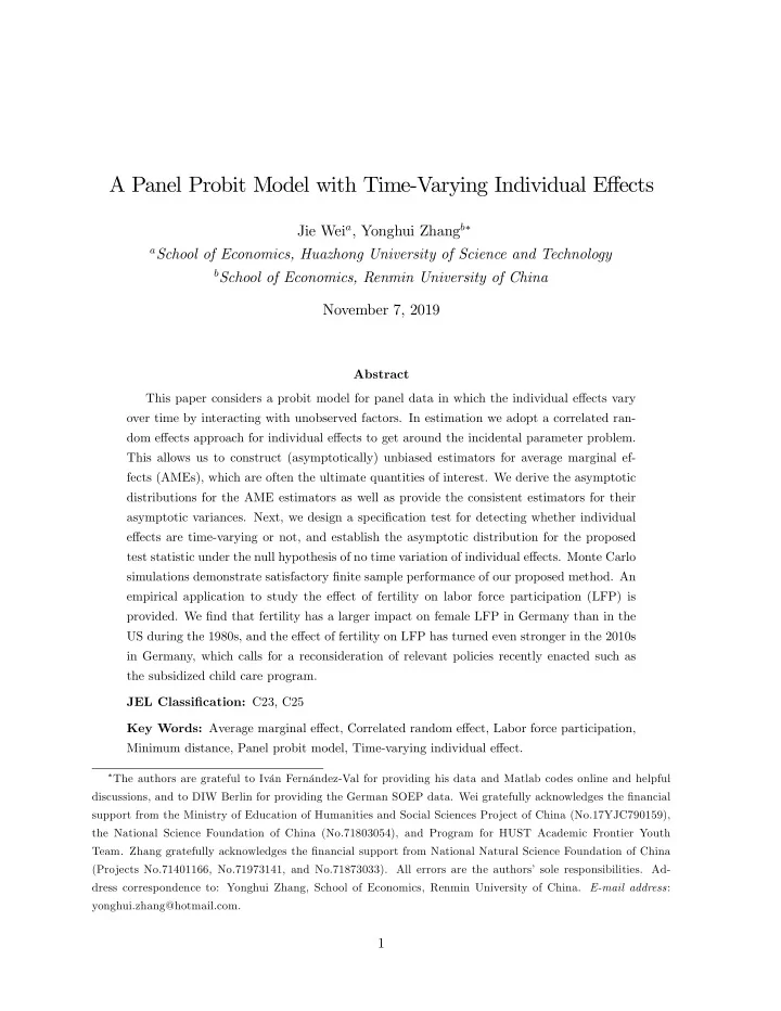
SLIDE 23 varies with her youngest child’s age on average, across the two sample periods of 1984-1988 and 2011-2017. On one hand, the LFP of women with children old enough has indeed increased noticeably from the 1980s to the 2010s; on the other hand, the job participation rate for a mother with a child aging 0-1 gets lower in the 2010s. Figure 3 shows how a new-born child a¤ects women LFP along time. It is clear that the di¤erence of LFP made by a new-born kid is getting larger from the 1980s to 2010s. Figures 2 and 3 both indicate a perhaps even stronger negative e¤ect of fertility on LFP more recently.
0-1 2-4 5-7 8-10 11-12 13-15 16-18 10 20 30 40 50 60 70 80 90
L F P ( % )
2011-2017 1984-1988
Figure 2: LFP and the youngest child’s age
1984 1985 1986 1987 1988 10 20 30 40 50 60 70 80 90
LF P (% )
2011 2012 2013 2014 2015 2016 2017 10 20 30 40 50 60 70 80 90
LF P (% )
Figure 3: LFP with and without a new-born child. Panel C in Table 7 further provides evidence more formally based on our proposed estimation
- method. It con…rms a signi…cant decrease of LFP due to fertility more recently, from about
23
SLIDE 24
21% in the 1980s to about 37% in the 2010s. Meanwhile, the e¤ects on LFP from older kids have not changed much by comparing Panels B and C. As in Panel B, other estimators tend to underestimate the AME of fertility in Panel C. The under-estimation can also be seen in estimating year-speci…c AMEs reported in part (C) of Figure 1. Again, this is not of surprise given the strong evidence of TVIE provided in column (C) of Table 6. Our empirical evidence in studying German SOEP during 2010-2017 suggests that, while more subsidized child care is accessible to women in Germany more recently, their LFP has not been encouraged but dropped instead. Several possible explanations for the ine¤ectiveness of subsidized child care in raising maternal labor supply are provided here. First, as noted by Blau and Robins (1988), unpaid child care (given by such as friends and relatives) is commonly used, which exhibits a negative impact on the mothers’ utility, and Havnes and Mogstad (2011) …nd that the new subsidized child care mostly crowds out unpaid (informal) child care arrangements, instead of increasing mothers’ labor supply. Second, a mother may not prefer subsidized care for her child below age two, because it is more expensive than for older kids, or because the mother perceives more important to spend time with her much younger kid (Bick, 2016). Besides, Baker et al. (2008) …nd that child care programs lead to children worse o¤ by measures ranging from aggression to motor and social skills to illness. Third, for mothers inclined to use paid child care, the access to subsidization lowers the relative price for the service. While a lower price of market child care makes it more appealing for mothers to go out for work, the associated income e¤ect may dominate and thus reduce their actual participation in jobs.
6 Conclusions
This paper studies a panel probit model with time-varying individual e¤ects under large N and …xed T. We propose asymptotically unbiased estimators for di¤erent AMEs, valid inference approaches, and also a speci…cation test for the presence of TVIE. We establish the asymptotic distribution for our estimators, and derive the limiting distribution of our speci…cation test under the null hypothesis of time-invariant individual e¤ects. Monte Carlo simulations demonstrate substantial gains in accuracy for the estimation by taking into account of the TVIE, and sat- isfactory …nite sample performance of the speci…cation test. An empirical application con…rms fertility as a key determinant of female labor force participation in the 1980s, with a larger impact in Germany than in the US. Evidence further shows that the (negative) dependence of labor participation on fertility has turned even stronger in Germany in the 2010s, which calls for a reconsideration of relevant policies recently enacted such as the subsidized child care program. References 24
SLIDE 25 Ahn, S., Lee, Y., and Schmidt, P., 2001. GMM estimation of linear panel data models with time-varying individual e¤ects. Journal of Econometrics 101, 219-255. Ahn, N., and Mira, P., 2002. A note on the changing relationship between fertility and female employment rates in developed countries. Journal of Population Economics 15(4), 667- 682. Anderson, P.M., and Levine, P.B., 1999. Child care and mothers’ employment decisions. Tech- nical Report. National Bureau of Economic Research. Ando, T. and Bai, J., 2018. Large scale panel choice models with unobserved heterogeneity: a Bayesian data augmentation approach. Working Paper. Angrist, J., 2001. Estimation of limited dependent variable models with dummy endogenous regressors: Simple strategies for empirical practice. Journal of Business & Economic Sta- tistics 19(1), 2-16. Angrist, J. and Evans, W., 1998. Children and their parents labor supply: Evidence from exogenous variation in family size. American Economic Review 88(3), 450-477. Attanasio, O., Low, H., and Sanchez-Marcos, V., 2008. Explaining changes in female labor supply in a life-cycle model. American Economic Review 98(4), 1517-1552. Baker, M., Gruber, J., and Milligan, K., 2008. Universal child care, maternal labor supply, and family well-being. Journal of Political Economy 116(4), 709-745. Bai, J., 2009. Panel data models with interactive e¤ects. Econometrica 77(4), 1229-1279. Bick, A., 2016. The quantitative role of child care for female labor force participation and
- fertility. Journal of the European Economic Association 14(3), 639-668.
Blau, D., Currie, J., 2006. Pre-school, day care, and after-school care: who’s minding the kids? In: Hanushek, E.A., and Welch, F. (Eds.), Handbook of the Economics of Education, vol. 2, Chapter 20. Blau, D., and Robins, F., 1988. Child-care costs and family labor supply. The Review of Economics and Statistics 70(3), 374-381. Boneva, L. and Linton, O., 2017. A discrete-choice model for large heterogeneous panels with interactive …xed e¤ects with an application to the determinants of corporate bond issuance. Journal of Applied Econometrics 32, 1226-1273. Bonhomme, S., and Manresa, E., 2015. Grouped patterns of heterogeneity in panel data. Econometrica 83(3), 1147-1184. Borck, R., 2014. Adieu Rabenmutter–culture, fertility, female labour supply, the gender wage gap and childcare. Journal of Population Economics 27(3), 739-765. Carrasco, R., 2001. Binary choice with binary endogenous regressors in panel data: Estimat- ing the e¤ect of fertility on female labor participation. Journal of Business & Economic Statistics 19(4), 385-394. Chamberlain, G., 1982. Multivariate regression models for panel data. Journal of Econometrics 18(1), 5-46. Chamberlain, G., 1984. Panel data. In: Griliches, Z., and Intriligator, M.(Eds.), Handbook of Econometrics, vol. 2, Chapter 22. Chen, M., Fernández-Val, I. and Weidner, M., 2019. Nonlinear factor models for network and panel data. Cemmap Working Paper, CWP18/19, The IFS. 25
SLIDE 26 Daniela, D.B., and Robert, M.S., 2009. Life cycle employment and fertility across institutional
- environments. European Economic Review 53, 274-292.
Domeij, D., Klein, P., 2013. Should day care be subsidized? The Review of Economic Studies 80(2), 568-595. European Council, 2002. Barcelona European Council. Presidency Conclusions, SN 100/1/02 REV 1. Fernández-Val, I., 2009. Fixed e¤ects estimation of structural parameters and marginal e¤ects in panel probit models. Journal of Econometrics 150, 71-85. Francesconi, M., 2002. A joint dynamic model of fertility and work of married women. Journal
- f Labor Economics 20, 336-380.
Haan, P., Wrohlich, K., 2011. Can child care policy encourage employment and fertility?: Evidence from a structural model. Labour Economics 18(4), 498-512. Hahn, J. and Newey W., 2004. Jackknife and analytical bias reduction for nonlinear panel
- models. Econometrica 72(4), 1295-1319.
Hausman, J., Hall, B., and Griliches, Z., 1984. Econometric models for count data with an application to the patents-R&D relationship. Econometrica 52(4), 909-938. Havnes, T., Mogstad, M., 2011. Money for nothing? Universal child care and maternal em-
- ployment. Journal of Public Economics 95(11), 1455-1465.
Heckman, J., 1974. E¤ects of child-care programs on women’s work e¤ort. Journal of Political Economy 82(2), 136-163. Holtz-Eakin, D., Newey, D., and Rosen, H., 1988. Estimating vector autoregressions with panel
- data. Econometrica 56, 1371-1395.
Hotz, V.J., and Miller, R., 1988. An empirical analysis of life cycle fertility and female labor
- supply. Econometrica 56, 91-118.
Hsiao, C., 2014. Analysis of Panel Data, 5th Edition. Cambridge University Press, Cambridge. Hsu, Y. and Shiu, J., 2019. Nonlinear panel data models with distribution-free correlated random e¤ects. Working Paper. Hwang, J., Park, S., and Shin, D., 2018. Two birds with one stone: Female labor supply, fertility, and market childcare. Journal of Economic Dynamics and Control 90, 171-193. Kögel, T., 2004. Did the association between fertility and female employment within OECD countries really change its sign? Journal of Population Economics 17(1), 45-65. Lefebvre, P., and Merrigan, P., 2008. Child-care policy and the labor supply of mothers with young children: A natural experiment from Canada. Journal of Labor Economics 26, 519-548. Michalopoulos, M., Robins, P., and Gar…nkel, I., 1992. A structural model of labor supply and child care demand. Journal of Human Resources 27(1), 166-203. Moon, H. and Weidner, M., 2015. Linear regression for panel with unknown number of factors as interactive …xed e¤ects. Econometrica 83(4), 1543-1579. Mundlak, Y., 1978. On the pooling of time series and cross section data. Econometrica 46(1), 69-85. 26
SLIDE 27
Newey, W., and McFadden, D., 1994. Large sample estimation and hypothesis testing. In: Engle, R., and McFadden, D.(Eds.), Handbook of Econometrics, vol. 4, Chapter 36. Pesaran, M., 2006. Estimation and inference in large heterogeneous panels with a multifactor error structure. Econometrica 74, 967-1012. Ribar, D., 1992. Child care and the labor supply of married women: reduced form evidence. Journal of Human Resources 27(1), 134-165. Tekin, E., 2007. Childcare subsidies, wages, and employment of single mothers. Journal of Human Resources 42, 453-487. White, H., 2001. Asymptotic Theory for Econometricians, Revised Edition. Academic Press. Wooldridge, J.M., 2010. Econometric Analysis of Cross Section and Panel Data, 2nd Edition. The MIT Press, Cambridge, Massachusetts. Wooldridge, J.M. and Zhu, Y., 2019. Inference in approximately sparse correlated random e¤ects probit models. Journal of Business & Economic Statistics, forthcoming. 27
SLIDE 28 APPENDIX
Recall that Wit
it;
X0
i
0, t
t; 0 t
0, qit 2Yit 1, ait (t)
qit(qitW 0
itt)
(qitW 0
itt) , and
HN;t (t)
1 N
PN
i=1 ait (t) (ait (t) + W 0 itt) WitW 0
- it. Now, we turn to the proof of Proposition
2.1. Proof of Proposition 2.1. Recall that ^ (^
- 1; ; ^
- T )0 is the estimator of (0
1; ; 0 T )0.
Using the Cramér-Wold Theorem, we complete the proof by showing that p N(^ )0C
d
! N(0; C0C) C0N(0; ) for any C (C0
1; ; C0 T )0 2 RT(2p+1) with Ct 2 R2p+1 for each t.
Denote the average of log likelihood function for the tth period observations evaluated at t by L(t), which takes the following form L(t) = 1 N
N
X
i=1
itt
itt
When Assumption 1 holds, by the standard theory of MLE (see, e.g., Newey and McFadden (1994)), we can show that: (i) ^ t = 0
t + op
for each t = 1; : : : ; T; and (ii) @2L(0
t )
@t@0
t =
Ht;N(0
t ) = Ht + op (1) for each t = 1; : : : ; T. By some simple calculation, we have
@L(t) @t = 1 N
N
X
i=1
YitWit (W 0
itt)
(W 0
itt)
(1 Yit) (W 0
itt) Wit
1 (W 0
itt)
N
N
X
i=1
Witait: Then by the …rst order conditions (FOCs) of MLE for probit model and the fact (i), we have p N
t 0
t
N;t(0 t )
p N @L(0
t )
@t + op (1) = 1 p N
N
X
i=1
H1
t
Wita0
it + op (1) ;
where we use the fact (ii) in the last equation. It follows that p N(b 0)0C = p N
T
X
t=1
t 0
t
Ct = 1 p N
N
X
i=1
&T;i (C) + op (1) where &T;i (C) PT
t=1 H1 t
a0
itW 0 itCt = PT t=1 '0 itCt = '0 iC with 'i = ('0 i1; ; '0 iT )0 and
'it = H1
t
a0
- itWit. Noting that &T;i (C)’s are independent across i, by verifying the Liapounov
condition, we can show that the Lindeberg-Feller central limit theorem (CLT) holds; see, e.g., Theorem 5.10 in White (2001). It follows that
1 p N
PN
i=1 &T;i (C) d
! N(0; C0C) by noting that limN!1 1
N
PN
i=1Var(&T;i (C)) = C0Var('i) C = C0C by the de…nition of in Proposition 2.1.
Proof of Theorem 2.2. Recall that it(t) = t(W 0
itt) and it = it(0 t ). Rewrite b
t =
1 N
PN
i=1 it(^
t) and 0
t = 1 N
PN
i=1 E (it). Let _
it (t) = it (t)Eit (t) ; i() =
iT (T )
0 ; _ it = it Eit and _ i = i
p N
= 1 p N
N
X
i=1
h i
= 1 p N
N
X
i=1
h i
+ 1 p N
N
X
i=1
_ i
28
SLIDE 29 For the …rst term AN1, by the Taylor expansion of Gi
- ^
- at the true value 0, we have
AN1 = " 1 N
N
X
i=1
@i
# p N
+ op (1) = D0p N
+ op (1) where we have used the fact that N1 PN
i=1 @i(0) @0
= D0 + op (1) in the last equation. By Proposition 2.1, we can show that AN1
d
! N
: For AN2, by the Lindeberge-Feller CLT for INID r.v.’s again, we have AN2
d
! N (0; ). By the fact that Xi and ui are mutually independent, it is straightforward to show that AN2 and AN1 are asymptotically uncorrelated. It follows that p N
0 d ! N
. Proof of Proposition 2.4. We complete the proof of the consistency by showing that for 8t; s = 1; : : : ; T, (i) ^ ts = ts+op (1), (ii) ^ D0
t = D0 t +op (1), and (iii) ^
ts = ts+op (1). We only prove (i) since the proofs for (ii) and (iii) are similar. Recall that ^ ts = 1
N
PN
i=1 it(^
t)is(^ s)0 h
1 N
PN
i=1 it(^
t) i h
1 N
PN
i=1 is(^
s)0i = ^ (1)
ts + ^
(2)
ts , say. Under Assumption 1, by the uniform
WLLN, we have ^ (1)
ts = E
is
(2)
ts = E (it) E
- is
- +op (1) for all t; s = 1; : : : ; T.
It follows that (i) holds. Proof of Theorem 3.1. We prove the theorem by using a result in Proposition 8 of Chamber- lain (1982). We …rst verify two assumptions (Assumptions 1-2) in Chamberlain (1982). Note that the almost sure convergence used in the assumptions can be weakened to convergence in probability, while keeping the conclusion still hold. First, under H0, = y = G(#). By Proposition 2.1, for the true value #0, we have ^ = G(#0) + op (1) and p N(^ G(#0))
d
! N(0; ). Second, by Proposition 2.4, ^ ts = ts + op (1) for t; s = 1; : : : ; T. It follows that ^ = + op (1) when T is …nite. This implies that ^ 1 = 1 + op (1) since the smallest eigenvalue of is bounded away from zero by Assumption 1. Third, let G(#) = @G(#)
@#0 , which can be written as
G(#) =
1 ; Cy0 2 )0; (y 01; ; y 0T )0 (02p1; I2p)0 T(1+2p)(T+2p) :
Apparently, rank[G(#)] = T + 2p is the dimension of #. Lastly, the second order derivatives (SOCs) of G(#) are all constants, and hence are certainly continuous. Then Assumptions 1-2 in Chamberlain (1982) hold. So we can apply Proposition 8 in Chamberlain (1982) to show that J
d
! 2
2(T1)p under H0 by noting that the degree of freedom is the number of restrictions
2(T 1)p. 29