a non standard model distrmod an s4 class based package
play

A non-standard model distrMod an S4 -class based package for - PowerPoint PPT Presentation

A non-standard model distrMod an S4 -class based package for statistical models one-dim. location scale model: X i i . i . d . P , = ( , ), L ( X i ) = L ( + v i ) p ( x ) e | x | 3 v i i . i . d .


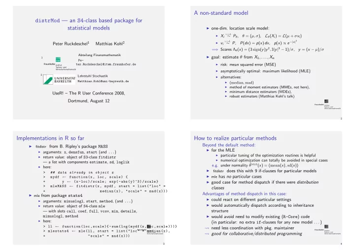
  1. A non-standard model distrMod — an S4 -class based package for statistical models ◮ one-dim. location scale model: ◮ X i i . i . d . ∼ P θ , θ = ( µ, σ ), L θ ( X i ) = L ( µ + σ v i ) p ( x ) ∝ e −| x | 3 ◮ v i i . i . d . Peter Ruckdeschel 1 Matthias Kohl 2 ∼ P , P ( dx ) = p ( x ) dx , ⇒ Scores Λ θ ( x ) = (3 sign ( y ) y 2 , 3 | y | 3 − 1) /σ , = y = ( x − µ ) /σ Abteilung Finanzmathematik ◮ goal: estimate θ from X 1 , . . . , X n 1 Pe- ◮ risk: mean squared error (MSE) ter.Ruckdeschel@itwm.fraunhofer.de ◮ asymptotically optimal: maximum likelihood (MLE) 2 Lehrstuhl Stochastik ◮ alternatives: Matthias.Kohl@uni-bayreuth.de ◮ ( median , mad ) ◮ method of moment estimators (MMEs, not here), ◮ minimum distance estimators (MDEs), UseR! – The R User Conference 2008, ◮ robust estimators (Matthias Kohl’s talk) Dortmund, August 12 2 Implementations in R so far How to realize particular methods Beyond the default method: fitdistr from B. Ripley’s package MASS ◮ ◮ for the MLE ◮ arguments: x , densfun , start (and ... ) ◮ particular tuning of the optimization routines is helpful ◮ return value: object of S3 -class fitdistr ◮ numerical optimization can totally be avoided in special cases — a list with components estimate , sd , loglik e.g. under normality ˆ θ MLE ( x ) = ( mean ( x ) , sd ( x )) ◮ here: fitdistr does this with 9 if-clauses for particular models ◮ > ## data already in object x ◮ mle has no particular cases > mydf ← function(x, loc , scale) { y ← (x-loc)/scale; exp(-abs(y)^3)/scale} ◮ good case for method dispatch if there were distribution + ← > mleMASS fitdistr(x, mydf , start = list("loc" = classes + median(x), "scale" = mad(x))) Advantages of method dispatch in this case: ◮ mle from package stats4 ◮ could react on different particular settings ◮ arguments: minuslogl , start , method , (and ... ) ◮ would automatically dispatch according to inheritance ◮ return value: object of S4 -class mle structure — with slots call , coef , full , vcov , min , details , minuslogl , method ◮ would avoid need to modify existing ( R-Core ) code ◮ here: (in particular: no extra if -clauses for any new model . . . ) ← > ll function(loc ,scale ){-sum(log(mydf(x,loc ,scale )))} � need less coordination with pkg. maintainer ← > mlestats4 mle(ll , start = list("loc" = median(x), � good for collaborative/distributed programming + "scale" = mad(x))) 3 4

  2. Packages for Distributions Classes distr : what is this good for? ◮ Problem: How to pass a distribution as an argument? arises e.g. in a function returning the population median The distrXXX Family of Packages ◮ lots of distributions already implemented to R naming convention: [ r,d,p,q ] <distr.name> for (Co-)Authors (besides M. Kohl) r RNG ◮ Thomas Stabla: statho3@web.de d density / probability function ◮ Florian Camphausen: fcampi@gmx.de p cdf q quantile function Organization in packages ◮ solution by eval , parse , paste ◮ distr , distrEx ; [and distrSim , distrTEst ] ← > mymedian function(distr , ...){ ◮ distrDoc , distrTeach , distrMod + eval(parse(text = paste( "x�=�q", distr , + "(1/2 ,...)", sep = ""))); return(x)} Availability ◮ better idea: having a“variable type” distribution ◮ published on CRAN ; current version 1.9 and functions p , d , q , r defined for this type ◮ devel version 2.0 on R-forge , r-forge.r-project.org ◮ i.e.: q (x) returns the quantile function � ← > median function(X){q(X)(0.5)} = ⇒ Development of this concept in package distr 5 6 Concept of R-Packages distr Methods Distribution (distr) Arithmetics for distributions r : function ◮ automatic generation of image distributions (of r.v.’s) d : OptionalFunction p : OptionalFunction q : OptionalFunction � overloaded operators "+" , "-" , "*" , "/" , "^" img : rSpace param : OptionalParameter ◮ group math of unary math. op.’s available, i.e., sin , exp , . . . e.g. Y ← (3 ✯ X ✯ Z+5) / 4 —generates L ( Y ) for Y = (3 XZ + 5) / 4 UnivariateDistribution (distr) UnivariateCondDistribution MultivariateDistribution simil.: exp ( sin (3 ✯ X+5) / 4) cond : Condition AbscontDistribution (distr) DiscreteDistribution (distr) DiscreteMVDistribution Implementation details support : numeric support : matrix ◮ binary operators interpret operands as stoch. independent AbscontCondDistribution DiscreteCondDistribution Gumbel support : numeric ◮ default simulation-based method for filling slots d , p , q ◮ AbscontDistribtion → Beta , Cauchy , Chisq , Exp , Fd , ◮ default FFT-based convolution methods for two indep. r.v.’s; Gammad , Logis , Lnorm , Norm , Td , Unif , Weibull c.f. K., R., & Stabla[04] ◮ DiscreteDistribtion → Binom , Dirac , Geom , Hyper , ◮ by method dispatch: use of analytic expressions Nbinom , Pois (. . . all from stats package) — e.g. N ( µ 1 , σ 2 1 ) ∗ N ( µ 2 , σ 2 2 ) = N ( µ 1 + µ 2 , σ 2 1 + σ 2 2 ) ◮ particular methods for plot , show , summary ,. . . ◮ distributions with non-trivial discrete and (abs.)continuous part ◮ easy generating functions DiscreteDistribution () , realized as mixing distributions AbscontDistribution () ◮ classes for mixing distributions 7 8

  3. Example Example Distribution Plot for mymix > ### generate some distribution mymix cdf of mymix quantile fct of mymix ← > wg flat.mix( UnivarMixingDistribution (Unif (0,1), Unif (4,5), ● 5 ● 0.8 ● ● ● 4 + withSimplify=FALSE )) ● ● ● ● 3 p(q) q(p) ● ● 0.4 ● ● ← 2 > mymix UnivarLebDecDistribution (acPart = wg , ● ● 1 ● 0.0 ● + discretePart = Binom (4,.4), acWeight = 0.4) ● 0 0 1 2 3 4 5 0.0 0.2 0.4 0.6 0.8 1.0 > #slots r,p,q: q p > r(mymix )(5) ## RNG density of ac.part(mymix) cdf of ac.part(mymix) quantile fct of ac.part(mymix) [1] 0.7672470 0.9290900 4.0000000 2.0000000 0.4746638 5 0.4 0.8 ● 4 > p(mymix )(c(0 ,1.2 ,3.2)) ## cdf ● ● 3 d(x) p(q) q(p) 0.2 0.4 ● ● 2 [1] 0.07776 0.48512 0.78464 ● 1 0.0 0.0 > q(mymix )((0:4)/4) ## quartiles 0 0 1 2 3 4 5 0 1 2 3 4 5 0.0 0.2 0.4 0.6 0.8 1.0 [1] 0.000000 0.861200 1.571420 3.124360 5.000000 x q p > #some new distribution as image law under trafo density of discrete part(mymix) cdf of discrete part(mymix) quantile fct of discrete part(mymix) > (mnew ← mymix*Norm (0 ,2)+3) # output shortened ● ● ● ● 4 ● ● ● ● 0.30 0.8 ● ● ● ● ● 3 An object of class "AffLinUnivarLebDecDistribution" d(x) p(q) q(p) ● ● 0.15 ● ● ● 2 ● 0.4 ● --- a Lebesgue decomposed distribution: ● ● 1 ● ● ● ● 0.0 0.00 ● ● ● ● 0 0 1 2 3 4 −1 0 1 2 3 4 5 0.0 0.2 0.4 0.6 0.8 1.0 Its discrete part (with weight 0.078000) is a[...] x q p Its absolutely continuous part (with weight 0.922000) is a[...] > plot(mymix) 9 10 Package distrEx Models in the distrXXX -family: package distrMod ◮ general expectation operator ◮ new class L2ParamFamily with slots ◮ functionals on distributions like ◮ distribution of the observations ◮ parameter median, var, sd, MAD and IQR ◮ L 2 -derivative Λ θ ( x ) and Fisher information I θ ◮ distances between distributions ◮ to“move” P θ from θ to θ ′ : functional slots realizing maps (e.g. Kolmogoroff–, Total-Variation–, Hellinger-distance) ◮ (factorized) conditional distributions and expectations θ �→ I θ , θ �→ Λ θ ( x ) , θ �→ P θ Example: Expectation Operator ◮ subclass L2LocationScaleFamily ◮ for a normal variable D 1 try to realize E D 1 , E D 2 1 ◮ generating function L2LocationScaleFamily() > D1 ← Norm ( mean =2) ◮ ## generation of distribution with density ∝ e −| x | 3 > m1 ← E(D1) # = 2 function ( x ) { xˆ2 } ) # E ( D 2 > myD ← AbscontDistribution (d = function(x){ > E(D1 , 1 ) + exp(-abs(x)^3)} , withS = TRUE) ◮ now —without changing the code— the same for a Poisson ## generating some data (already run earlier) variable; � same calls but different dispatched methods > x ← r(myD )(40) > D1 ← ## generation of L2Family Pois ( lambda =3) > m1 ← E(D1) ← # = 3 > myDF L2LocationScaleFamily (centraldistr = myD) > E(D1 , function ( x ) { xˆ2 } ) > plot(myDF) 11 12

Download Presentation
Download Policy: The content available on the website is offered to you 'AS IS' for your personal information and use only. It cannot be commercialized, licensed, or distributed on other websites without prior consent from the author. To download a presentation, simply click this link. If you encounter any difficulties during the download process, it's possible that the publisher has removed the file from their server.

Recommend


More recommend