A Monte Carlo Based Response Matrix Method for Pin-wise Transport - - PDF document

SLIDE 1

A Monte Carlo Based Response Matrix Method for Pin-wise Transport Calculations

Sori Jeon, Namjae Choi, Han Gyu Joo* Department of Nuclear Engineering, Seoul National University, 1 Gwanak-ro, Gwanak-gu, Seoul, 08826 Korea

*Corresponding author: joohan@snu.ac.kr

• 1. Introduction

The response matrix method (RMM) is a famous two- step calculation method which would enable fast core transport calculation based on pre-generated response

• matrices. Due to its advantage that no homogenization is

necessary, it once had stood as a compelling method for whole-core transport calculations. However, as the deterministic transport methods such as the method of characteristics (MOC) have become relatively cheap to be directly applied to the core analyses while providing much higher flexibility, RMM had gradually fallen out

• f interest.

However, RMM may stand out again in the modern trend of computing processor technology development. As artificial intelligence (AI) and big data industries which require a tremendous amount of computing power are experiencing a significant growth, the processors are also being specialized to the operations used in those fields which involves large dense matrix operations. For example, a single GeForce RTX 2080 Ti GPU, which is consumer grade, is capable of delivering up to 110 TFLOPS of the matrix – matrix multiplication performance through the specialized tensor cores. It is equivalent to more than a thousand cores of typical server-grade CPU processors. In this regard, we suggest an RMM formulation using the Monte Carlo (MC) method. The calculation of response matrices with MC was introduced in the direct response matrix (DRM) method of HITACHI [1] and the COMET code [2], and both works demonstrated promising results. In their works, however, the response matrices are fixed to an assembly configuration, which limits the flexibility. Therefore, we introduce a pin-wise RMM and examine its feasibility.

• 2. Response Matrix Method

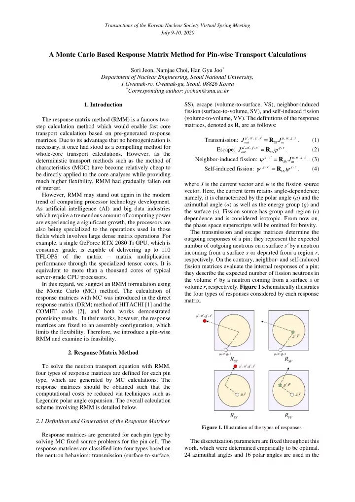
To solve the neutron transport equation with RMM, four types of response matrices are defined for each pin type, which are generated by MC calculations. The response matrices should be obtained such that the computational costs be reduced via techniques such as Legendre polar angle expansion. The overall calculation scheme involving RMM is detailed below. 2.1 Definition and Generation of the Response Matrices Response matrices are generated for each pin type by solving MC fixed source problems for the pin cell. The response matrices are classified into four types based on the neutron behaviors: transmission (surface-to-surface, SS), escape (volume-to-surface, VS), neighbor-induced fission (surface-to-volume, SV), and self-induced fission (volume-to-volume, VV). The definitions of the response matrices, denoted as R, are as follows: Transmission:

, , , , , , ' ' g' s' g s

• ut

SS in

J J

   

 R

. (1) Escape:

, , , , ' ' g' s' g r

• ut

VS

J     R

. (2) Neighbor-induced fission:

, , , , g' r' g s SV in

J     R

. (3) Self-induced fission:

, , g' r' g r VV

   R

. (4) where J is the current vector and ψ is the fission source

• vector. Here, the current term retains angle-dependence;

namely, it is characterized by the polar angle (μ) and the azimuthal angle (α) as well as the energy group (g) and the surface (s). Fission source has group and region (r) dependence and is considered isotropic. From now on, the phase space superscripts will be omitted for brevity. The transmission and escape matrices determine the

• utgoing responses of a pin; they represent the expected

number of outgoing neutrons on a surface s′ by a neutron incoming from a surface s or departed from a region r,

• respectively. On the contrary, neighbor- and self-induced

fission matrices evaluate the internal responses of a pin; they describe the expected number of fission neutrons in the volume r′ by a neutron coming from a surface s or volume r, respectively. Figure 1 schematically illustrates the four types of responses considered by each response matrix.

Figure 1. Illustration of the types of responses

The discretization parameters are fixed throughout this work, which were determined empirically to be optimal. 24 azimuthal angles and 16 polar angles are used in the

Transactions of the Korean Nuclear Society Virtual Spring Meeting July 9-10, 2020

SLIDE 2

hemisphere on each surface; due to axial symmetry, only upper 12 azimuthal angles are considered. Each side of a pin is divided into three surfaces and the fuel consists of regions divided by three rings and four azimuthal sectors. Figure 2 illustrates the discretization structure of a pin.

Figure 2. Discretization of a pin

The response matrix generation procedure with MC is as follows:

• 1. Depending on whether the response matrix to generate

is current-induced or source-induced, the neutrons are uniformly created either on a surface (s) or in a region (r) with isotropic angle (μ, α) and random energy (g). The number of input neutrons created in each bin of phase space is scored at ( , , , )

S

I g s  

• r

( , )

V

I g r .

• 2. Each neutron is simulated until it reaches a surface.

Neutron weights are reduced by implicit capture but Russian roulette is not used.

• 3. If a neutron escapes a surface (s′) with angle (μ′, α′)

and energy (g′), its weight is scored: ( , , , , , , )

SS SS

g s g s w            R R , (5) ( , , , , )

VS VS g r

g s w          R R . (6)

• 4. If a neutron undergoes a fission reaction in a region (r′)

and produces ν neutrons with energy (g′), the yield is scored: ( , , , , )

SV SV

g s g r         R R , (7) ( , , )

VV VV g r

g r       R R . (8)

• 5. Once all the neutrons are traced, the scored responses

are divided by the input neutron scores to obtain unit responses, which becomes the response matrices: ( , , , ) / ( , , , )

SS SS S

g s I g s      R R , (9) ( , ) / ( , )

VS VS V

g r I g r  R R , (10) ( , , , ) / ( , , , )

SV SV S

g s I g s      R R , (11) ( , ) / ( , )

VV VV V

g r I g r  R R . (12) 2.2 Legendre Polar Angle Expansion In RMM, most of the computing time is spent for the transmission calculation; namely, multiplication of RSS and Jin. As can be easily inferred, RSS is the largest matrix

• ut of the four types of the response matrices. If all the

variables are incorporated into the matrix in a discretized form, the dimension of the matrix easily reaches tens of

• thousands. This results in an impractical memory usage

and computing time as the multiplication is repeatedly

• performed. Therefore, it is necessary to take a measure

to reduce the size of the matrix. In this regard, a polar angle expansion technique based

• n Shifted Legendre Polynomials (SLP) is introduced. It

can reduce the number of polar angle components in the matrix from the number of polar angles to the number of moments which is determined by the expansion order. In principle, sufficient number of polar angles must be used for accuracy because it has large impact on the reactivity due to the self-shielding effect. However, it was observed that the distribution of current in μ shows fairly smooth behavior so that it can be adequately fitted by low-order

• polynomials. In this work, 2nd order expansion is chosen,

and therefore only 3 coefficients are required to express the polar angle dependence of current as follows:

2

( ) ( )

l l l

J J P  



  , (13) where Pl is the l-th order SLP and

l

J is the l-th moment.

In accordance with the expansion, we need to tally the polar angle moments of the outgoing neutrons. It can be achieved by the MC functional expansion tally technique. The orthogonality of SLP yields the following relation between the moment and the current:

1

(2 1) ( ) ( )

l

• ut
• ut

l

J l J P d       . (14) Thus, by simply scoring (2l + 1)Pl(μ) for each outgoing neutron, the response in terms of moments can be tallied. Resultantly, the transmission equation is reformulated as follows:

• ut

SS in

J J  R P , (15) where

SS

R is a modified transmission matrix that gives the moments as the response for the incoming currents, and P is a conversion matrix that calculates the physical currents from the moments, whose entries are merely the piece-wise integrals of the SLPs:

1

( )

i i

ij j

P P d

 

 



  . (16) In actual calculations,

SS

R P , which is much smaller than the original transmission matrix RSS, is used as the single response matrix and the currents are carried in the moment form. Note that the equations for the escape response and the neighbor-induced fission response should be modified as well:

• ut

VS

J   R , (17)

SV in

J   R P . (18) In the same manner, RSVP is stored as a single response matrix. 2.3 CMFD Acceleration As a fission source convergence acceleration scheme, CMFD acceleration is introduced to RMM. However, as RMM neither calculates flux nor employs cross sections which are necessary to calculate the homogenized group constants, response matrices for the flux and the reaction rates are also calculated by the procedure analogous to the primary response matrices.

Transactions of the Korean Nuclear Society Virtual Spring Meeting July 9-10, 2020

SLIDE 3

The definition of the response matrices for the flux and the reaction rates are as follows:

x S in

x J  R P , (19)

x V

x   R

. (20) where x is the desired quantity which is pin-homogenized, and

x S

R ,

x V

R are current- and source-induced response matrices of x, respectively. Once the pin-homogenized flux and reaction rates are

• btained throughout the RMM iteration, group constants

can be calculated and CMFD acceleration can be carried

• ut. The response matrices for the CMFD acceleration

are small and does not add much computational overhead to the main RMM procedure. 2.4 Power Iteration Scheme The algorithm for solving the k-eigenvalue problem with RMM is presented in Figure 3. First, the response contributions of the initial fission sources are calculated, namely [1] the escape response that gives initial currents

• n the surfaces and [2] the self-induced fission response.

It is followed by the inner iteration which [3] iteratively updates the currents on the surfaces by the transmission response and [4] accumulates the fission sources for the next outer iteration step by the neighbor-induced fission

• response. Note that at each inner iteration step, every pin

has to receive the outgoing currents of the adjacent pins and update its own incoming currents, which also adds a certain amount of overhead. Accumulation of the CMFD quantities is also done in appropriate locations. The inner iteration is continued until the currents are fully attenuated. Once the inner iteration had converged, the remaining procedures are analogous to the ordinary power iteration incorporating CMFD acceleration.

OUTER : DO WHILE Not Converged [1] Escape:

• ut

VS

J   R [2] Self-induced fission:

VV

   R Accumulate source-induced flux and reaction rates INNER : DO WHILE

• ut

J   Update

in

J using

• ut

J [3] Transmission:

• ut

SS in

J J  R P [4] Neighbor-induced fission:

SV in

J     R P Accumulate current-induced flux and reaction rates Accumulate surface net currents END DO INNER Update eigenvalue Check convergence Perform CMFD acceleration and update  Save old fission source:    END DO OUTER Figure 3. Power iteration algorithm

• 3. Results

In this section, accuracy and performance of RMM are evaluated by a comparative study with the MOC solver

• f nTRACER [3]. An MC code PRAGMA [4] is used as

the reference. The problems are based on the C5G7MOX benchmark problem but manipulated in some degree to discover the distinction of RMM from the conventional MOC solver. The nTRACER calculations were carried

• ut with 0.01cm ray spacing and 16/4 azimuthal/polar

angles were used in octant. 3.1 Single Assembly Calculations Here, five types of assemblies are examined whose configurations are shown in Figure 4. A1 and A2 are the

• rdinary UO2 and MOX fuel assemblies of the

benchmark, and I1 to I3 are the variations which contain highly concentrated absorbers that mimic the integrated fuel burnable absorber (IFBA). The IFBA-like absorbers were designed by coating the control rod material in the benchmark on the surface of the fuel rods with 0.001cm

• thickness. The absorption cross sections of the control

rod material were then increased by 40 times. IFBA is the typical weak point of MOC which suffers from the ray effects; as the IFBA regions are way much thinner than the ‘beams’ represented by the rays, reaction rates in the IFBA region are highly biased. On the other hand, RMM captures the MC physics and theoretically it can handle any problems that the MC method can solve. Table 1 shows the eigenvalues of the assemblies and the errors of each method. The PRAGMA results were

• btained using 10 billion histories. As expected, RMM

reveals its strength in handling nonconventional problems that MOC cannot solve properly. A peculiar error in A2 of RMM still requires investigations. It is, however, clearly seen that the accuracy of RMM is not affected by the existence of IFBA while MOC shows large discrepancy. The error in I3 of RMM is caused by the baseline error of A2 and it is not due to IFBA itself.

Figure 4. Configurations of the single assembly problems Table 1. Eigenvalues of the single assembly problems

Case PRAGMA Δkeff (pcm) RMM MOC A1 1.33344 (1)

• 13

17 A2 1.18565 (1)

• 91
• 1

I1 1.07529 (1)

• 17
• 203

I2 0.95271 (1)

• 12
• 272

I3 1.05076 (1)

• 96
• 111

Transactions of the Korean Nuclear Society Virtual Spring Meeting July 9-10, 2020

SLIDE 4

3.2 2D Core Calculations A fictitious core loaded with I1 and I3 assemblies was designed to verify the core analysis capability of RMM, as described in Figure 5. Table 2 summarizes the results

• f eigenvalue and pin power errors, and the relative error

distributions of pin powers are shown in Figure 6. Both codes used 10-5 convergence criteria for the relative norm

• f fission source change, and the MC reference solution

was generated with 50 billion histories. Although the two codes have comparable pin power RMS errors, RMM does not show any power tilt that is present in the MOC solution. In addition, RMM captures the transport effect better which occurs at the material interfaces such as fuel – moderator and UO2 – MOX. The reactivity is also better estimated by RMM.

Figure 5. Configuration of the IFBA-bearing fictitious core Table 2. Calculation results of the 2D core.

Case keff Δkeff (pcm)

• Max. Rel.

∆P (%) RMS (%) PRAGMA 1.05673

• RMM

1.05626

• 47

1.34 0.24 MOC 1.05522

• 151

1.85 0.26

Figure 6. Relative error distributions of MOC and RMM

Nonetheless, the large computing time is the major drawback of RMM. Table 3 compares the computing time of RMM and nTRACER, which were executed on 20 cores of Intel Xeon E5-2630 v4 CPUs. In RMM, calculation of RSS and RSV, namely the inner iteration, contributes 75% and 20% to the total computing time, respectively, which leads to twice larger computing time than nTRACER. It should be addressed to retain the feasibility of pin-wise RMM.

Table 3. Comparison of total computing time

Code RMM nTRACER Computing Time (s) 2194.8 1031.4

• 4. Conclusions

An MC-based pin-wise response matrix method was introduced as a unique neutron transport solution scheme. The response matrices are generated for each pin type from fixed-source MC calculations. A polar angle expansion scheme using shifted Legendre polynomials was devised to reduce the computational cost and the CMFD acceleration was introduced in the response matrix framework. Since the response matrices are calculated by an MC code, RMM can reflect all the MC physics inside a pin. This strength was clearly observed in the verification results for the fictitious IFBA-bearing assemblies made from the C5G7MOX benchmark problem. While MOC suffered from large reactivity errors due to the ray effect, RMM could accurately capture the effect of IFBA. Also for the IFBA-bearing fictitious core, RMM performed better than MOC; the power tilt was eliminated and the transports effect appearing at the material interfaces were better captured, as well as having lower reactivity error. Still, substantive improvements are required for RMM. First of all, high computational cost has to be addressed by introducing more extensive expansions of variables. Especially, energy expansion is critical as expressing the continuous energy physics with the ordinary multi-group formulation will likely result in an impractical number of energy groups. In addition, problems with T/H feedback

• r depletion, in which the cross sections are continuously

varied, should be considered. ACKNOWLEDGMENTS

This work was supported by KOREA HYDRO & NUCLEAR POWER CO., LTD (No. 2018-Tech-09).

REFERENCES

[1] M. Moriwaki, K. Ishii, H. Maruyama, M. Aoyama, “A New Direct Calculation Method of Response Matrices Using a Monte Carlo Calculation,” Journal of Nuclear Science and Technology 36(3), pp. 877-887 (1999). [2] B. Forget, “A Three Dimensional Heterogeneous Coarse Mesh Transport Method for Reactor Calculations,” Ph.D. Dissertation, Georgia Institute of Technology (2006). [3] Y. S. Jung, C. B. Shim, C. H. Lim, H. G. Joo, “Practical Numerical Reactor Employing Direct Whole Core Neutron Transport and Subchannel Thermal/Hydraulics Solvers,” Annals of Nuclear Energy 62, pp. 357-374 (2013). [4] N. Choi, K. M. Kim, H. G. Joo, “Initial Development of PRAGMA – A GPU-Based Continuous Energy Monte Carlo Code for Practical Applications” Proceedings of the Korean Nuclear Society Autumn Meeting, Goyang, Korea,

• Oct. 24-25 (2019).

I1 I3 I1 I3 I1 I3 I1 I3 I3 I1 I3 I1 I3 I1 I3 I1 I1 I3 I1 I3 I1 I3 I1 I3 I3 I1 I3 I1 I3 I1 I3 I1 I3 I1 I3 I1 I3 I1 I3 I1 I3 I1 I3 I1 I1 I3 I1 I3 I1 I3 I1 I3

Transactions of the Korean Nuclear Society Virtual Spring Meeting July 9-10, 2020