A distributed approximation scheme for sleep scheduling in sensor - - PowerPoint PPT Presentation

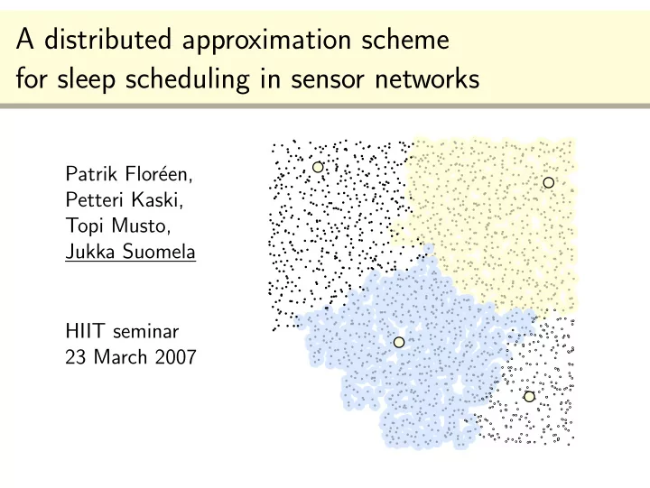
A distributed approximation scheme for sleep scheduling in sensor networks

Patrik Flor´ een, Petteri Kaski, Topi Musto, Jukka Suomela HIIT seminar 23 March 2007

A sensor network

Battery-powered sensor devices Maximise the lifetime by letting each node sleep occasionally

2 / 32

Pairwise redundancy relations

Two sensors close to each other may be pairwise redundant If v is active then u can be asleep and vice versa

Detecting pairwise redundancy: e.g., Koushanfar et al. (2006)

v u

3 / 32

Redundancy graph for the sensor network

All pairwise redundancy relations

4 / 32

A dominating set in the redundancy graph

If v1 is active then its neighbours can be asleep v1

5 / 32

A dominating set in the redundancy graph

If v2 is active then its neighbours can be asleep v1 v2

6 / 32

A dominating set in the redundancy graph

If v3 is active then its neighbours can be asleep v1 v2 v3

7 / 32

A dominating set in the redundancy graph

If nodes {v1, v2, v3} are active then all other nodes can be asleep

• D = {v1, v2, v3} is

a dominating set in this redundancy graph v1 v2 v3

8 / 32

Sleep scheduling in sensor networks

Task: find multiple dominating sets and apply them one after another Objective: maximise total lifetime Constraints: the battery capacity of each node

9 / 32

Domatic partition

One approach: find disjoint dominating sets Achieved lifetime: 2 time units Each node active for 1 time unit Feasible but not optimal! 1 time unit 1 time unit

10 / 32

Fractional domatic partition

1 2 units 1 2 units 1 2 units 1 2 units 1 2 units 5 2 time units

Each node active for 1 time unit Achieved lifetime:

11 / 32

Towards the distributed algorithm

Optimal sleep scheduling =

• ptimal fractional domatic partition

◮ Hard to optimise and hard to

approximate in general graphs

◮ Centralised solutions are not

practical in large networks Plan:

◮ Identify the features of

typical redundancy graphs

◮ Exploit the features to design a

distributed approximation scheme

1 2 units 1 2 units

· · ·

12 / 32

Construction of a typical redundancy graph

A potato field

13 / 32

Construction of a typical redundancy graph

Planting sensors. . .

14 / 32

Construction of a typical redundancy graph

Planting sensors. . .

15 / 32

Construction of a typical redundancy graph

Planting sensors. . .

16 / 32

Construction of a typical redundancy graph

A sensor network

17 / 32

Construction of a typical redundancy graph

Wireless communication links

18 / 32

Construction of a typical redundancy graph

Wireless communication links Some example nodes highlighted

Not necessarily a unit disk graph

19 / 32

Construction of a typical redundancy graph

Redundancy relations An arbitrary subgraph of the communication graph

Nodes that can communicate with each other can also determine whether they are pairwise redundant

20 / 32

Construction of a typical redundancy graph

The complete redundancy graph

In this example: approx. 2000 nodes 6000 redundancy edges 100000 communication links (not shown)

21 / 32

Features of a typical redundancy graph (1)

Bounded density of nodes

Cover a larger area = ⇒ still at most N sensors in any unit disk

22 / 32

Features of a typical redundancy graph (2)

Bounded length of edges In the communication graph and thus also in the redundancy graph

Limited range of radio, limited range of sensor

23 / 32

Features of a typical redundancy graph (3)

The communication graph is a geometric spanner A shortest path in the graph is not much longer than the shortest path in the plane

“Sensible” network topology; here guaranteed by the deployment process No such assumption is made about the redundancy graph

24 / 32

Features of a typical redundancy graph

Communication graph

• 1. Density of nodes
• 2. Length of edges
• 3. Geometric

spanner Redundancy graph

◮ Any subgraph

Given these assumptions, there exists a distributed approximation scheme

25 / 32

The distributed approximation scheme

Idea 1:

• 1. Partition the graph into small cells
• 2. Solve the scheduling problem

locally in each cell

◮ Nodes near a cell boundary

help in domination

◮ Local optimum at least

as good as global optimum

• 3. Merge the local solutions

Problem:

◮ Nodes near a cell boundary

work suboptimally

26 / 32

The distributed approximation scheme

Idea 2: shifting strategy

(e.g., Hochbaum & Maass 1985)

• 1. Form several partitions
• 2. Make sure no node is near

a cell boundary too often

• 3. Construct a schedule for each

partition and interleave Works fine if the nodes know their coordinates Can we form the partitions without using any coordinates ?

27 / 32

The distributed approximation scheme

Install anchor nodes

Or use a distributed algorithm to find suitable anchors: e.g., any maximal independent set in a power graph of the communication graph

Not too sparse, not too dense 1 bit of information: “I am an anchor”

28 / 32

The distributed approximation scheme

Finding one partition is now easy: Voronoi cells for anchors

◮ Metric: hop counts in communication graph

How do we get more partitions? No global consensus

• n left/right,

north/south

29 / 32

The distributed approximation scheme

Assumption: locally unique identifiers for anchors

◮ MAC addresses ◮ Random numbers

Shift borders towards those anchors with larger identifiers

Key lemma

No node is near a cell boundary too often

30 / 32

The distributed approximation scheme

A constant number of partitions suffices Cell size is constant

Main result

For any ǫ > 0, with suitable anchor placement, sleep scheduling can be approximated within 1 + ǫ in constant time per node

31 / 32

Summary

◮ Sleep scheduling in sensor networks

= fractional domatic partition

◮ Formalise the features which make

the problem easier to approximate

◮ Anchors suffice, coordinates are

not needed

◮ A distributed approximation

scheme, constant effort per node

◮ Demonstrates theoretical feasibility

– more work needed to make the constants practical To appear in Proc. SECON 2007

1 2 units 1 2 units

· · ·

32 / 32