= [ [ ] ] = ( ( ) ) A A A A m i j , + + + + < - PDF document

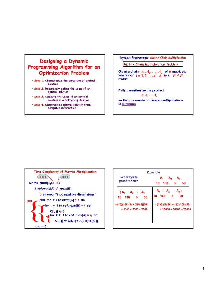
Dynamic Programming: Matrix Chain Multiplication Designing a Dynamic Designing a Dynamic Matrix Chain Multiplication Problem Programming Algorithm for an Programming Algorithm for an Optimization Problem … Optimization Problem n Given a chain of matrices, A A , , , A × 1 2 n = p p … where (for ) is a i 1,2, , n A i i i matrix • Step 1. Step 1. Characterize the structure of optimal Characterize the structure of optimal • solution solution • • Step 2. Step 2. Recursively define the value of an Recursively define the value of an Fully parenthesize the product optimal solution optimal solution � A A A • Step 3. Step 3. Compute the value of an optimal Compute the value of an optimal • 1 2 n solution in a bottom- solution in a bottom -up fashion up fashion so that the number of scalar multiplications • Step 4. • Step 4. Construct an optimal solution from Construct an optimal solution from is minimum minimum computed information computed information Time Complexity of Matrix Multiplication Time Complexity of Matrix Multiplication Example p x q q x r Two ways to A 1 A 2 A 3 parenthesize Matrix-Multiply(A, B) 10 100 5 50 ≠ if columns [A] rows [B] A 1 ( A 2 A 3 ) ( A 1 A 2 ) A 3 then error “incompatible dimensions” 10 100 5 50 10 100 5 50 else for i � 1 to rows [A] = p do pqr { { { = (10)(100)(5) + (10)(5)(50) = (100)(5)(50) + (10)(100)(50) for j � 1 to columns [B] = r do rq = 5000 + 2500 = 7500 = 25000 + 50000 = 75000 C[I, j] � 0 for k � 1 to columns [A] = q do q C[I, j] � C[I, j] + A[I, k]*B[k, j] return C 1

P n = A A A A Let number of ways to parenthesize a Can be parenthesized in 5 ways ( ) 1 2 3 4 product of n matrices, then ( ( ) ) ( ( ) ) ( ( ) ) A A A A =  1 2 3 4 1 if n 1  ( ( ) ) ( ( ( ( ) ) ) ) =  P n ( ) n A A A A  ∑ − − ≥ ≥ 1 2 3 4 P k P n ( ) ( k ) if n 2  ( ( ( ( ) ( ) ( ) ) ) ) = k 1 A A A A 1 2 3 4 = = − − It can be shown that , P n ( ) C n ( 1) ( ( ) ) ( ( ) ) C n − ( ( ) ) where is the (n-1)-th Catalan ( 1) A A A A 1 2 3 4 number ( ( ) ) ( ( ) ) ( ( ) )     n 2 n 1 4 A A A A = = = Ω = C n ( )     1 2 3 4 +    3/ 2  n 1 n n = Notation � Objective A A A A … + i j i i 1 j [ [ ] ] m i j = Min # of mult. to evaluate A … , i j Find a way to fully parenthesize the product =  0 if i j  = [ [ ] ] � =  ( ( ) ) A A A A m i j , + + + + < min m m p p p if i j …   1 n 1 2 n + + − − i k , k 1, j i 1 k j ≤ ≤ ≤ ≤ i k j in such a way that the cost is minimum [ [ ] ] s i j = that k such that , [ [ ] ] [ ] [ ] = = + + + + m i j , m i k , m k 1, j p p p − i 1 k j 2

• Optimal Substruc. Property ( --- ) ( --- ) • Overlapping Subproblems Property Recursive formula for m[I, j] leads to an exponential problem Observation: Relatively few problems Set of problems { i…j } So # of subprobs. is the # of ways of ≤ ≤ ≤ ≤ ≤ choosing I, j such that , 1 i j n  ⇒   + n which is Overlap   n  2 ( )( ) ( ) ( ) 3

Analysis of Recursive- Analysis of Recursive -Matrix Matrix- -Chain Chain T n = time to compute optimal parenth. of ( ) chain of n matrices ≥  T (1) 1   − n 1 ∑ ( ( ) ) ≥ ≥ + + + − + > T n ( ) 1 T k ( ) T n ( k ) 1 for n 1   = k 1 ≥ � − � − Assuming the Induction hypothesis 1 n 1 T ( ) 2 ∑ ( ( ) ) ≥ ≥ + + + − + T ( n ) 1 T ( k ) T ( n k ) 1 for , we have: ≤ ≤ − − � n 1 = k 1 − n 1 ∑ = = + + 2 T ( k ) n = − − − − k 1 n 1 n 2 ∑ ∑ ≥ ≥ − + + = + We use math induction to prove that k 1 k T n ( ) 2 2 n 2 2 n ( ( ) ) T n = Ω = Ω = = = = 2 n k 1 k 0 ( ) ( ( ) ) = = − − − + = − + n 1 n 2 2 1 n 2 2 n The basis step is easy: − ≥ n 1 2 ≥ ≥ = = 0 T (1) 1 2 4

Memoization Memoization Memoization Memoization • Create a table for solns to subprobs so far computed • Initialize each table entry to a symbol indicating subprob not yet computed • Each time a subproblem is first encountered, its soln is computed and placed in the table • Each subsequent time it is encountered, its previously computed soln is simply retrieved from the table How to Design a Dynamic Prog Prog. Algorithm . Algorithm How to Design a Dynamic Prog Prog. Algorithm . Algorithm How to Design a Dynamic How to Design a Dynamic 1. Identify the subproblems – 3. Apply “generic dynamic prog. algorithm – • Subprobs must be of same type as original probs • Use bottom-up version • Subprobs must be smaller • use top-down version (Memoization) • How to specify each subprob? • What is the base case? What is the recursive case? 4. Modify your algorithm to compute 2. Characterize the op. soln as a combination description of soln to value of soln, if needed of op solns to subprobs – • Add additional table • Focus on value of soln rather than description of soln • Introduce notation to rep. value of op soln to each subprob • Consider trying all possible solns to prob 5

Longest Common Subsequence (LCS) Longest Common Subsequence (LCS) Longest Common Subsequence Longest Common Subsequence (LCS) (LCS) = … Def. A seq is a subseq of Z z z , , z { 1 2, k = X A B C B D A B , , , , , , = If … if there is a strictly X x x , , x 1 2, n = increasing seq … of the indices of Y B D C A B A , , , , , i i , , , k i X 1 2 such that = x z then common subsequences are, for i j j example, LCS Problem: Given two seqs, find an LCS and BCA BCBA Both are common subsequences (CS). But = … Notation: Given , the i-th X x x , , x only the last is a LCS. 1 2, n prefix is defined as the subseq X i … x x , , x 1 2, i Thm 16 (p351). (Optimal substructure of LCS) So … So … =  …  Let be seqs, X x x , , , x  1 2 m  = …   Y y , y , , y 1 2 n ( ( ) ) = = = = … and let , then Z z z , , , z LCS X Y , ? = 1 2 k x y m n ( ( ) ) NO Yes 1. and = = ⇒ = = = = Z LC S X , Y x y z x y − − − − − k 1 m 1 n 1 m n k m n = = = = z x y k m n ? ≠  x y & m n  ⇒ 2. . ( ( ) ) ( ( ) ) ≠ ≠ =  = z x z y & Z L C S X , Y Z LC S X , Y − − − − − − k m k n m 1 k 1 m 1 n 1  ≠ z x  & & k m ( ( ) ) ( ( ) ) = = ≠ Z LCS X , Y Z LCS X Y − ,  3. . − x y m 1 n 1 m n  ⇒ ( ( ) ) =  & Z L C S X , Y − n 1  ≠  z y k n 6

Notation Notation ( ( ) ) [ [ ] ] c i j = Length of LCS X Y , , i j  = = = = 0 if i 0 or j 0  [ [ ] ] [ ] = = − − − + > =  c i j , c i 1 , j 1 1 if i j , 0& x y i j  ( ( [ [ ] [ ] [ ] ] ) ) − − − − > ≠ M ax c i j , 1 , c i 1 , j if i j , 0& x y  i j [ [ ] ] [ [ ] ] … … points to the entry of c 0 i ,0 j b i j , corresponding to the optimal subprob soln [ [ ] ] chosen when computing c i j , 7