
SLIDE 1
CSCI 621: Digital Geometry Processing
Hao Li
http://cs621.hao-li.com
1
Spring 2019
7.2 Surface Reconstruction Hao Li http://cs621.hao-li.com 1 - - PowerPoint PPT Presentation
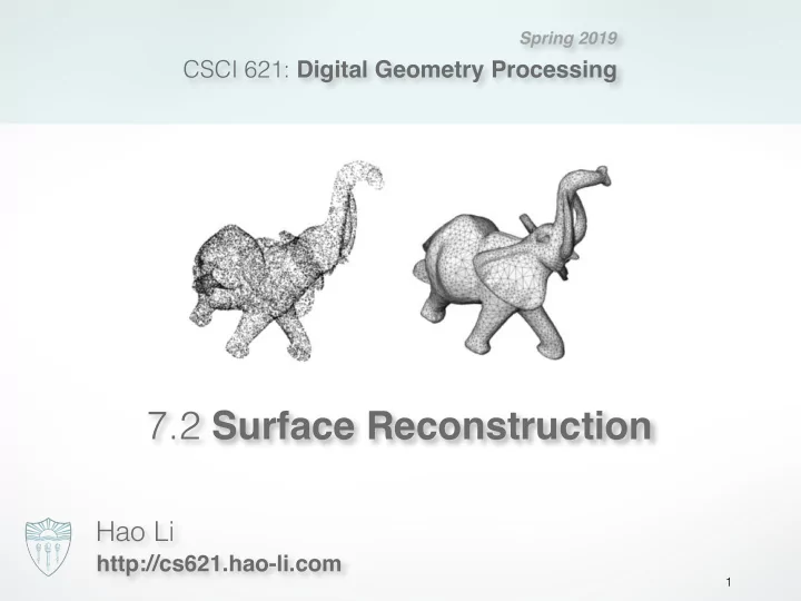
Spring 2019 CSCI 621: Digital Geometry Processing 7.2 Surface Reconstruction Hao Li http://cs621.hao-li.com 1 Surface Reconstruction physical captured reconstructed model point cloud model 2 Input Data Set of irregular sample points
CSCI 621: Digital Geometry Processing
http://cs621.hao-li.com
1
Spring 2019
2
physical model captured point cloud reconstructed model
3
range scan vertices
mesh
through local connectivity
Given a set of points P = {p1, . . . , pn} with pi ∈ R3
Find a manifold surface S ⊂ R3 which approximates P
Local surface connectivity estimation Point interpolation Signed distance function estimation Mesh approximation
– Ball pivoting algorithm – Delaunay triangulation – Alpha shapes – Zippering... – Distance from tangent planes – SDF estimation via RBF – ... – Image space triangulation
Given a set of points P = {p1, . . . , pn} with pi ∈ R3 Find a manifold surface S ⊂ R3 which approximates P where S = {x | d(x) = 0} with d(x) a signed distance function
Point cloud Signed distance function estimation Evaluation of distances on uniform grid Mesh extraction via marching cubes Mesh
d(x) d(i), i = [i, j, k] ∈ Z3
Mainly differ in their signed distance function
13
14
15
16
17
18
19
explicit implicit input model
20
21
22
23
24
25
26
27
m
i=1
28
E(c, n) =
m
⇤
i=1
⇥2 =
m
⇤
i=1
pi ⇥2 (with ˆ pi := pi − c) =
m
⇤
i=1
ˆ pT
i nnT ˆ
pi (version 1) =
m
⇤
i=1
nT ˆ piˆ pT
i n
(version 2)
29
∂E(c, n) ∂c =
m
−2 nnT ˆ pi = −2 nnT
m
ˆ pi
!
= 0
m
ˆ pi = 0 ⇒ c = 1 m
m
pi
30
1 + α2 2 + α2 3
nT Cn = α2
1λ1 + α2 2λ2 + α2 3λ3 ≥ α2 1λ3 + α2 2λ3 + α2 3λ3 = λ3
31
32
m
m
33
34
i nj < 0
i nj|
35
36
37
150 samples reconstruction
38
39
dist(xj) =
n
wi · ϕ(⇤xj ci⇤)
!
= dj, j = 1, . . . , n
ϕ(⇤x1 x1⇤) · · · ϕ(⇤x1 xn⇤) . . . ... . . . ϕ(⇤xn x1⇤) · · · ϕ(⇤xn xn⇤) w1 . . . wn = d1 . . . dn
+
Hoppe ‘92 Compact RBF Wendland C2
⇤ I R
3
∂3dist ∂x ∂x ∂x ⇥2 + ∂3dist ∂x ∂x ∂y ⇥2 + · · · + ∂3dist ∂z ∂z ∂z ⇥2 dx dy dz → min
Hoppe ‘92 Compact RBF Wendland C2 Global RBF Triharmonic
45
46
47
48
d1 d2 w1 w2 w1+w2 (w1d1+w2d2)/(w1+w2)
SDFs Weight Functions
[Curless,Levoy96]
[Curless,Levoy96]
49
50
[Curless,Levoy96]
51
4G sample points → 8M triangles 1G sample points → 8M triangles
52
53
SIGGRAPH 1992
radial basis functions, SIGGRAPH 2001
Models from Range Images, SIGGRAPH 1996.
Statues, SIGGRAPH 2000.
54
55
56
the shape
Indicator function
57
Indicator function Oriented points
58
Oriented points
Indicator gradient
59
χ kr ~
60
χ kr ~
61
62
63
64
65
66
67
68
69
70
71
72
73
scans
Time (s) / Peak Memory (MB) 200 400 600 800 Triangles 175,000 350,000 525,000 700,000 Time Taken Peak Memory Usage
Power Crust FastRBF MPU VRIP FFT Reconstruction Poisson Reconstruction
83
Surface Smoothing
84