6 INTRODUCTION TO MULTIVARIABLE CONTROL [3] 6.1 Transfer - - PDF document

6 INTRODUCTION TO MULTIVARIABLE CONTROL [3]

6.1 Transfer functions for MIMO systems [3.2]

✲ G1 ✲ G2 ✲ G u z

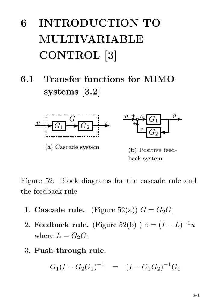
(a) Cascade system

✲❜✲ + + G1 ✲ ♣ ✛ G2 ✻ u y v z

(b) Positive feed- back system

Figure 52: Block diagrams for the cascade rule and the feedback rule

• 1. Cascade rule. (Figure 52(a)) G = G2G1
• 2. Feedback rule. (Figure 52(b) ) v = (I − L)−1u

where L = G2G1

• 3. Push-through rule.

G1(I − G2G1)−1 = (I − G1G2)−1G1

6-1

MIMO Rule: Start from the output, move

• backwards. If you exit from a feedback loop then

include a term (I − L)−1 where L is the transfer function around that loop (evaluated against the signal flow starting at the point of exit from the loop). Example

z = (P11 + P12K(I − P22K)−1P21)w (6.1)

❝ ❝ q ✲ ❄ ✲ ✛ ✲ ❄ ✲ ✲ ✲ ✲

+ + + + z P12 P11 P22 K P21 w

Figure 53: Block diagram corresponding to (6.1)

6-2

Negative feedback control systems ✲ ❝ ✲ +

• K

✲ ❝ + + ❄✲ G ✲ ❝ + + ❄ ✲ q ✻ r y u d2 d1 Figure 54: Conventional negative feedback control system

• L is the loop transfer function when breaking the

loop at the output of the plant. L = GK (6.2) Accordingly S

∆

= (I + L)−1

• utput sensitivity

(6.3) T

∆

= I − S = (I + L)−1L = L(I + L)−1

• utput complementary sensitivity(6.4)

LO ≡ L, SO ≡ S and TO ≡ T.

6-3

• LI is the loop transfer function at the input to

the plant LI = KG (6.5) Input sensitivity: SI

∆

= (I + LI)−1 Input complementary sensitivity: TI

∆

= I − SI = LI(I + LI)−1

• Some relationships:

(I + L)−1 + (I + L)−1L = S + T = I (6.6) G(I + KG)−1 = (I + GK)−1G (6.7) GK(I+GK)−1 = G(I+KG)−1K = (I+GK)−1GK (6.8) T = L(I + L)−1 = (I + L−1)−1 = (I + L)−1L (6.9) Rule to remember: “G comes first and then G and K alternate in sequence”.

6-4

6.2 Multivariable frequency response analysis [3.3]

G(s) = transfer (function) matrix G(jω) = complex matrix representing response to sinusoidal signal of frequency ω ✲ ✲ y G(s) d Figure 55: System G(s) with input d and output y y(s) = G(s)d(s) (6.10)

6-5

Sinusoidal input to channel j dj(t) = dj0 sin(ωt + αj) (6.11) starting at t = −∞. Output in channel i is a sinusoid with the same frequency yi(t) = yi0 sin(ωt + βi) (6.12) Amplification (gain): yio djo = |gij(jω)| (6.13) Phase shift: βi − αj = gij(jω) (6.14) gij(jω) represents the sinusoidal response from input j to output i.

6-6

Example 2 × 2 multivariable system, sinusoidal signals of the same frequency ω to the two input channels: d(t) = d1(t) d2(t)

• =

d10 sin(ωt + α1) d20 sin(ωt + α2)

• (6.15)

The output signal y(t) = y1(t) y2(t)

• =

y10 sin(ωt + β1) y20 sin(ωt + β2)

• (6.16)

can be computed by multiplying the complex matrix G(jω) by the complex vector d(ω): y(ω) = G(jω)d(ω) y(ω) = y10ejβ1 y20ejβ2

• , d(ω) =

d10ejα1 d20ejα2

• (6.17)

6-7

6.2.1 Directions in multivariable systems [3.3.2] SISO system (y = Gd): gain |y(ω)| |d(ω)| = |G(jω)d(ω)| |d(ω)| = |G(jω)| The gain depends on ω, but is independent of |d(ω)|. MIMO system: input and output are vectors. ⇒ need to “sum up” magnitudes of elements in each vector by use of some norm d(ω)2 =

• j

|dj(ω)|2 =

• d2

10 + d2 20 + · · · (6.18)

y(ω)2 =

• i

|yi(ω)|2 =

• y2

10 + y2 20 + · · · (6.19)

The gain of the system G(s) is y(ω)2 d(ω)2 = G(jω)d(ω)2 d(ω)2 =

• y2

10 + y2 20 + · · ·

• d2

10 + d2 20 + · · ·

(6.20) The gain depends on ω, and is independent of d(ω)2. However, for a MIMO system the gain depends on the direction of the input d.

6-8

Example Consider the five inputs ( all d2 = 1)

d1 =

1

• , d2 =

1

• , d3 =

0.707

0.707

• ,

d4 =

0.707

−0.707

• , d5 =

0.6

−0.8

• For the 2 × 2 system

G1 =

• 5

4 3 2

• (6.21)

The five inputs dj lead to the following output vectors y1 =

5

3

• , y2 =

4

2

• , y3 =

6.36

3.54

• , y4 =

0.707

0.707

• , y5 =

−0.2

0.2

• with the 2-norms (i.e. the gains for the five inputs)

y12 = 5.83, y22 = 4.47, y32 = 7.30, y42 = 1.00, y52 = 0.28

6-9

−5 −4 −3 −2 −1 1 2 3 4 5 2 4 6 8

y2/d2 d20/d10 ¯ σ(G1) = 7.34 σ(G1) = 0.27

Figure 56: Gain G1d2/d2 as a function of d20/d10 for G1 in (6.21) The maximum value of the gain in (6.20) as the direction of the input is varied, is the maximum singular value of G, max

d=0

Gd2 d2 = max

d2=1 Gd2 = ¯

σ(G) (6.22) whereas the minimum gain is the minimum singular value of G, min

d=0

Gd2 d2 = min

d2=1 Gd2 = σ(G)

(6.23)

6-10

−1 −0.5 0.5 1 −1 −0.5 0.5 1 −5 5 −4 −3 −2 −1 1 2 3 4

¯ σ(G) σ(G) ¯ v v y10 y20 d10 d20

Figure 1: Outputs (right plot) resulting from use of d2 = 1 (unit circle in left plot) for system G. The maximum (¯ σ(G)) and minimum (σ(G)) gains are ob- tained for d = (¯ v) and d = (v) respectively.

1-8

6.2.2 Eigenvalues are a poor measure of gain [3.3.3] Example G = 100

• ;

G 1

• =

100

• (6.24)

Both eigenvalues are equal to zero, but gain is equal to 100. Problem: eigenvalues measure the gain for the special case when the inputs and the outputs are in the same direction (in the direction of the eigenvectors). For generalizations of |G| when G is a matrix, we need the concept of a matrix norm, denoted G. Two important properties: triangle inequality G1 + G2 ≤ G1 + G2 (6.25) and the multiplicative property G1G2 ≤ G1 · G2 (6.26) ρ(G)

∆

= |λmax(G)| (the spectral radius), does not satisfy the properties of a matrix norm

6-11

6.2.3 Singular value decomposition [3.3.4] Any matrix G may be decomposed into its singular value decomposition, G = UΣV H (6.27) where Σ is an l × m matrix with k = min{l, m} non-negative singular values, σi, arranged in descending order along its main diagonal; U is an l × l unitary matrix of output singular vectors, ui, V is an m × m unitary matrix of input singular vectors, vi, Example SVD of a real 2 × 2 matrix can always be written as G = cos θ1 − sin θ1 sin θ1 cos θ1

• U

σ1 σ2

• Σ

cos θ2 ± sin θ2 − sin θ2 ± cos θ2 T

• V T

(6.28) U and V involve rotations and their columns are

• rthonormal.

6-12

Input and output directions. The column vectors of U, denoted ui, represent the

• utput directions of the plant. They are orthogonal

and of unit length (orthonormal), that is ui2 =

• |ui1|2 + |ui2|2 + . . . + |uil|2 = 1

(6.29) uH

i ui = 1,

uH

i uj = 0,

i = j (6.30) The column vectors of V , denoted vi, are orthogonal and of unit length, and represent the input directions. Gvi = σiui (6.31) If we consider an input in the direction vi, then the

• utput is in the direction ui. Since vi2 = 1 and

ui2 = 1 σi gives the gain of the matrix G in this direction. σi(G) = Gvi2 = Gvi2 vi2 (6.32)

6-13

Maximum and minimum singular values. The largest gain for any input direction is ¯ σ(G) ≡ σ1(G) = max

d=0

Gd2 d2 = Gv12 v12 (6.33) The smallest gain for any input direction is σ(G) ≡ σk(G) = min

d=0

Gd2 d2 = Gvk2 vk2 (6.34) where k = min{l, m}. For any vector d we have σ(G) ≤ Gd2 d2 ≤ ¯ σ(G) (6.35) Define u1 = ¯ u, v1 = ¯ v, uk = u and vk = v. Then G¯ v = ¯ σ¯ u, Gv = σ u (6.36) ¯ v corresponds to the input direction with largest amplification, and ¯ u is the corresponding output direction in which the inputs are most effective. The directions involving ¯ v and ¯ u are sometimes referred to as the “strongest”, “high-gain” or “most important” directions.

6-14

Example

G1 =

• 5

4 3 2

• (6.37)

The singular value decomposition of G1 is G1 =

• 0.872

0.490 0.490 −0.872

• U
• 7.343

0.272

• Σ
• 0.794

−0.608 0.608 0.794

H

• V H

The largest gain of 7.343 is for an input in the direction ¯ v =

0.794

0.608

• , the smallest gain of 0.272 is for an input in

the direction v =

−0.608

0.794

• . Since in (6.37) both inputs

affect both outputs, we say that the system is interactive. The system is ill-conditioned, that is, some combinations

• f the inputs have a strong effect on the outputs, whereas
• ther combinations have a weak effect on the outputs.

Quantified by the condition number; ¯ σ/σ = 7.343/0.272 = 27.0. Example Shopping cart. Consider a shopping cart (supermarket trolley) with fixed wheels which we may want to move in three directions; forwards, sideways and upwards. For the shopping cart the gain depends strongly on the input direction, i.e. the plant is ill-conditioned.

6-15

Example: Distillation process.

Steady-state model of a distillation column G =

• 87.8

−86.4 108.2 −109.6

• (6.38)

Since the elements are much larger than 1 in magnitude there should be no problems with input constraints. However, the gain in the low-gain direction is only just above 1. G =

• 0.625

−0.781 0.781 0.625

• U
• 197.2

1.39

• Σ
• 0.707

−0.708 −0.708 −0.707

H

• V H

(6.39) The distillation process is ill-conditioned, and the condition number is 197.2/1.39 = 141.7. For dynamic systems the singular values and their associated directions vary with frequency (Figure 57).

6-16

10

−2

10 10

2

10

−1

10 10

1

10

2

Magnitude Frequency [rad/s] ¯ σ(G) σ(G) (a) Spinning satellite in (6.44)

10

−4

10

−2

10 10

−2

10 10

2

Magnitude Frequency [rad/s] ¯ σ(G) σ(G) (b) Distillation process in (6.49)

Figure 57: Typical plots of singular values

6-17

6.2.4 Singular values for performance [3.3.5] Maximum singular value is very useful in terms of frequency-domain performance and robustness. Performance measure for SISO systems: |e(ω)|/|r(ω)| = |S(jω)| . Generalization for MIMO systems e(ω)2/r(ω)2 σ(S(jω)) ≤ e(ω)2 r(ω)2 ≤ ¯ σ(S(jω)) (6.40) For performance we want the gain e(ω)2/r(ω)2 small for any direction of r(ω) ¯ σ(S(jω)) < 1/|wP (jω)|, ∀ω ⇔ ¯ σ(wP S) < 1, ∀ω ⇔ wP S∞ < 1 (6.41) where the H∞ norm is defined as the peak of the maximum singular value of the frequency response M(s)∞

∆

= max

ω

¯ σ(M(jω)) (6.42)

6-18

Typical singular values of S(jω) in Figure 58.

10

−2

10 10

2

10

−2

10

Magnitude Frequency [rad/s] Design 1: Design 2: σ(S) σ(S) ¯ σ(S) ¯ σ(S)

Figure 58: Singular values of S for a 2 × 2 plant with RHP-zero

• Bandwidth, ωB: frequency where ¯

σ(S) crosses

1 √ 2 = 0.7 from below.

Since S = (I + L)−1, the singular values inequality σ(A) − 1 ≤

1 ¯ σ(I+A)−1 ≤ σ(A) + 1 yields

σ(L) − 1 ≤ 1 ¯ σ(S) ≤ σ(L) + 1 (6.43)

• low ω : σ(L) ≫ 1 ⇒ ¯

σ(S) ≈

1 σ(L)

• high ω: ¯

σ(L) ≪ 1 ⇒ ¯ σ(S) ≈ 1

6-19

5.4 Poles [4.4]

Definition

• Poles. The poles pi of a system with state-space

description (5.1)–(5.2) are the eigenvalues λi(A), i = 1, . . . , n of the matrix A. The pole or characteristic polynomial φ(s) is defined as φ(s)

∆

= det(sI − A) = n

i=1(s − pi). Thus the poles

are the roots of the characteristic equation φ(s)

∆

= det(sI − A) = 0 (5.36) 5.4.1 Poles and stability Theorem 6 A linear dynamic system ˙ x = Ax + Bu is stable if and only if all the poles are in the open left-half plane (LHP), that is, Re{λi(A)} < 0, ∀i. A matrix A with such a property is said to be “stable”

• r Hurwitz.

5.4.2 Poles from transfer functions Theorem 7 The pole polynomial φ(s) corresponding to a minimal realization of a system with transfer function G(s), is the least common denominator of all non-identically-zero minors of all orders of G(s).

5-18

Example: G(s) = 1 1.25(s + 1)(s + 2) s − 1 s −6 s − 2

• (5.37)

The minors of order 1 are the four elements all have (s + 1)(s + 2) in the denominator. Minor of order 2 det G(s) = (s − 1)(s − 2) + 6s 1.252(s + 1)2(s + 2)2 = 1 1.252(s + 1)(s + 2) (5.38) Least common denominator of all the minors: φ(s) = (s + 1)(s + 2) (5.39) Minimal realization has two poles: s = −1; s = −2. Example: Consider the 2 × 3 system, with 3 inputs and

2 outputs, G(s) = 1 (s + 1)(s + 2)(s − 1)∗ ∗

• (s − 1)(s + 2)

(s − 1)2 −(s + 1)(s + 2) (s − 1)(s + 1) (s − 1)(s + 1)

• (5.40)

Minors of order 1: 1 s + 1, s − 1 (s + 1)(s + 2), −1 s − 1, 1 s + 2, 1 s + 2 (5.41)

5-19

Minor of order 2 corresponding to the deletion of column 2: M2 = (s − 1)(s + 2)(s − 1)(s + 1) + (s + 1)(s + 2)(s − 1)2 ((s + 1)(s + 2)(s − 1))2 = = 2 (s + 1)(s + 2) (5.42) The other two minors of order two are M1 = −(s − 1) (s + 1)(s + 2)2 , M3 = 1 (s + 1)(s + 2) (5.43) Least common denominator: φ(s) = (s + 1)(s + 2)2(s − 1) (5.44) The system therefore has four poles: s = −1, s = 1 and two at s = −2. Note MIMO-poles are essentially the poles of the

• elements. A procedure is needed to determine

multiplicity.

5-20

5.5 Zeros [4.5]

• SISO system: zeros zi are the solutions to

G(zi) = 0. In general, zeros are values of s at which G(s) loses rank. Example

• Y =

s + 2 s2 + 7s + 12U

• Compute the response when

u(t) = e−2t, y(0) = 0, ˙ y(0) = −1 L{u(t)} = 1 s + 2 s2Y − sy(0) − ˙ y(0) + 7sY − 7y(0) + 12Y = 1 s2Y + 7sY + 12Y + 1 = 1 ⇒ Y (s) = 0 Assumption: g(s) has a zero z, g(z) = 0. Then for input u(t) = u0ezt the output is y(t) ≡ 0, t > 0. (with appropriate initial conditions)

5-21

5.5.2 Zeros from transfer functions [4.5.2] Definition

• Zeros. zi is a zero of G(s) if the rank
• f G(zi) is less than the normal rank of G(s). The

zero polynomial is defined as z(s) = nz

i=1(s − zi)

where nz is the number of finite zeros of G(s). Theorem The zero polynomial z(s), corresponding to a minimal realization of the system, is the greatest common divisor of all the numerators of all order-r minors of G(s), where r is the normal rank of G(s), provided that these minors have been adjusted in such a way as to have the pole polynomial φ(s) as their denominators. Example

G(s) = 1 s + 2

• s − 1

4 4.5 2(s − 1)

• (5.45)

The normal rank of G(s) is 2. Minor of order 2: det G(s) = 2(s−1)2−18

(s+2)2

= 2 s−4

s+2.

Pole polynomial: φ(s) = s + 2. Zero polynomial: z(s) = s − 4.

Note Multivariable zeros have no relationship with the zeros of the transfer function elements.

5-23

Example G(s) = 1 1.25(s + 1)(s + 2) s − 1 s −6 s − 2

• (5.46)

Minor of order 2 is the determinant det G(s) = (s − 1)(s − 2) + 6s 1.252(s + 1)2(s + 2)2 = 1 1.252(s + 1)(s + 2) (5.47) φ(s) = 1.252(s + 1)(s + 2) Zero polynomial = numerator of (5.47) ⇒ no multivariable zeros. Example G(s) = s − 1 s + 1 s − 2 s + 2

• (5.48)
• The normal rank of G(s) is 1
• no value of s for which G(s) = 0

⇒ G(s) has no zeros.

5-24

5.6 More on poles and zeros[4.6]

5.6.1 *Directions of poles and zeros Let G(s) = C(sI − A)−1B + D. Zero directions. Let G(s) have a zero at s = z. Then G(s) loses rank at s = z, and there exist non-zero vectors uz and yz such that G(z)uz = 0, yH

z G(z) = 0

(5.49) uz = input zero direction yz = output zero direction yz gives information about which output (or combination of outputs) may be difficult to control. SVD: G(z) = UΣV H uz = last column in V yz = last column of U (corresponding to the zero singular value of G(z)) Pole directions. Let G(s) have a pole at s = p. Then G(p) is infinite, and we may write G(p)up = ∞, yH

p G(p) = ∞

(5.50) up = input pole direction yp = output pole direction.

5-25

Example Plant in (5.45) has a RHP-zero at z = 4 and a LHP-pole at p = −2. G(z) = G(4) = 1 6 3 4 4.5 6

• =

1 6 0.55 −0.83 0.83 0.55 9.01 0.6 −0.8 0.8 0.6 H uz = −0.80

0.60

• yz =

−0.83

0.55

• (5.51)

For pole directions consider G(p + ǫ) = G(−2 + ǫ) = 1 ǫ2 −3 + ǫ 4 4.5 2(−3 + ǫ)

• (5.52)

The SVD as ǫ → 0 yields G(−2+ǫ) = 1 ǫ2 −0.55 −0.83 0.83 −0.55 9.01 0.6 −0.8 −0.8 −0.6 H up = 0.60

−0.80

• yp =

−0.55

0.83

• (5.53)

Note Locations of poles and zeros are independent

• f input and output scalings, their directions are not.

5-26

5.6.2 Remarks on poles and zeros [4.6.2]

• 1. For square systems the poles and zeros of G(s)

are “essentially” the poles and zeros of det G(s). This fails when zero and pole in different parts of the system cancel when forming det G(s). G(s) = (s + 2)/(s + 1) (s + 1)/(s + 2)

• (5.54)

det G(s) = 1, although the system obviously has poles at −1 and −2 and (multivariable) zeros at −1 and −2.

• 2. System (5.54) has poles and zeros at the same

locations (at −1 and −2). Their directions are

• different. They do not cancel or otherwise

interact.

• 3. There are no zeros if the outputs contain direct

information about all the states; that is, if from y we can directly obtain x (e.g. C = I and D = 0);

• 4. Zeros usually appear when there are fewer inputs
• r outputs than states

5-27

• 5. Moving poles. (a) feedback control

(G(I + KG)−1) moves the poles, (b) series compensation (GK, feedforward control) can cancel poles in G by placing zeros in K (but not move them), and (c) parallel compensation (G + K) cannot affect the poles in G.

• 6. Moving zeros. (a) With feedback, the zeros of

G(I + KG)−1 are the zeros of G plus the poles of

• K. , i.e. the zeros are unaffected by feedback.

(b) Series compensation can counter the effect of zeros in G by placing poles in K to cancel them, but cancellations are not possible for RHP-zeros due to internal stability (see Section 5.7). (c) The only way to move zeros is by parallel compensation, y = (G + K)u, which, if y is a physical output, can only be accomplished by adding an extra input (actuator).

5-28

Example Effect of feedback on poles and zeros. SISO plant G(s) = z(s)/φ(s) and K(s) = k. T(s) = L(s) 1 + L(s) = kG(s) 1 + kG(s) = kz(s) φ(s) + kz(s) = k zcl(s) φcl(s) (5.55) Note the following:

• 1. Zero polynomial: zcl(s) = z(s)

⇒ zero locations are unchanged.

• 2. Pole locations are changed by feedback.

For example, k → 0 ⇒ φcl(s) → φ(s) (5.56) k → ∞ ⇒ φcl(s) → z(s). z(s) (5.57) where roots of z(s) move with k to infinity (complex pattern) (cf. root locus)

5-29

5.10 System norms [4.10]

✲ ✲ z w G Figure 51: System G

Figure 51: System with stable transfer function matrix G(s) and impulse response matrix g(t). Question: given information about the allowed input signals w(t), how large can the outputs z(t) become?

We use the 2-norm, z(t)2 =

• i

∞

−∞

|zi(τ)|2dτ (5.88) and consider three inputs:

• 1. w(t) is a series of unit impulses.
• 2. w(t) is any signal satisfying w(t)2 = 1.
• 3. w(t) is any signal satisfying w(t)2 = 1, but

w(t) = 0 for t ≥ 0, and we only measure z(t) for t ≥ 0. The relevant system norms in the three cases are the H2, H∞, and Hankel norms, respectively.

5-41

5.10.1 H2 norm [4.10.1] G(s) strictly proper. For the H2 norm we use the Frobenius norm spatially (for the matrix) and integrate over frequency, i.e. G(s)2

∆

=

• 1

2π ∞

−∞

tr(G(jω)HG(jω))

• G(jω)2

F = ij |Gij(jω)|2

dω (5.89) G(s) must be strictly proper, otherwise the H2 norm is infinite. By Parseval’s theorem, (5.89) is equal to the H2 norm of the impulse response G(s)2 = g(t)2

∆

=

• ∞

tr(gT (τ)g(τ))

• g(τ)2

F = ij |gij(τ)|2

dτ (5.90)

• Note that G(s) and g(t) are dynamic systems

while G(jω) and g(τ) are constant matrices (for a given value of ω or τ).

5-42

• We can change the order of integration and

summation in (5.90) to get G(s)2 = g(t)2 =

• ij

∞ |gij(τ)|2dτ (5.91) where gij(t) is the ij’th element of the impulse response matrix, g(t). Thus H2 norm can be

interpreted as the 2-norm output resulting from applying unit impulses δj(t) to each input, one after another (allowing the output to settle to zero before applying an impulse to the next input). Thus G(s)2 =

m

i=1 zi(t)2 2 where zi(t) is the output

vector resulting from applying a unit impulse δi(t) to the i’th input.

5-43

5.10.2 H∞ norm [4.10.2] G(s) proper. For the H∞ norm we use the singular value (induced 2-norm) spatially (for the matrix) and pick out the peak value as a function of frequency G(s)∞

∆

= max

ω

¯ σ(G(jω)) (5.93) The H∞ norm is the peak of the transfer function “magnitude”. Time domain performance interpretations of the H∞ norm.

• Worst-case steady-state gain for sinusoidal

inputs at any frequency.

• Induced (worst-case) 2-norm in the time domain:

G(s)∞ = max

w(t)=0

z(t)2 w(t)2 = max

w(t)2=1 z(t)2

(5.94) (In essence, (5.94) arises because the worst input signal w(t) is a sinusoid with frequency ω∗ and a direction which gives σ(G(jω∗)) as the maximum gain.)

5-45

Numerical computation of the H∞ norm. Consider G(s) = C(sI − A)−1B + D H∞ norm is the smallest value of γ such that the Hamiltonian matrix H has no eigenvalues on the imaginary axis, where H =

• A + BR−1DT C

BR−1BT −CT (I + DR−1DT )C −(A + BR−1DT C)T

• (5.95)

and R = γ2I − DTD 5.10.3 Difference between the H2 and H∞ norms Frobenius norm in terms of singular values G(s)2 =

• 1

2π ∞

−∞

• i

σ2

i (G(jω))dω

(5.96) Thus when optimizing performance in terms of the different norms:

• H∞: “push down peak of largest singular value”.
• H2: “push down whole thing” (all singular

values over all frequencies).

5-46

Example G(s) = 1 s + a (5.97) H2 norm: G(s)2 = ( 1 2π ∞

−∞

|G(jω)|2

• 1

ω2+a2

dω)

1 2

= ( 1 2πa

• tan−1(ω

a ) ∞

−∞)

1 2 =

• 1

2a Alternatively: Consider the impulse response g(t) = L−1

• 1

s + a

• = e−at, t ≥ 0

(5.98) to get g(t)2 = ∞ (e−at)2dt =

• 1

2a (5.99) as expected from Parseval’s theorem. H∞ norm: ||G(s)||∞ = max

ω

|G(jω)| = max

ω

1 (ω2 + a2)

1 2 = 1

a (5.100)

5-47

Example There is no general relationship between the H2 and H∞ norms. f1(s) = 1 ǫs + 1, f2(s) = ǫs s2 + ǫs + 1 (5.101) ||f1||∞ = 1 ||f1||2 = ∞ ||f2||∞ = 1 ||f2||2 = 0 (5.102) Why is the H∞ norm so popular? In robust control convenient for representing unstructured model uncertainty, and because it satisfies the multiplicative property: A(s)B(s)∞ ≤ A(s)∞ · B(s)∞ (5.103) What is wrong with the H2 norm? It is not an induced norm and does not satisfy the multiplicative property.

5-48

Example Consider again G(s) = 1/(s + a) in (5.97), for which G(s)2 =

• 1/2a.

G(s)G(s)2 =

• ∞

| L−1[( 1 s + a)2]

• te−at

|2 =

• 1

a 1 2a =

• 1

a G(s)2

2

(5.104) for a < 1, G(s)G(s)2 > G(s)2 · G(s)2 (5.105) which does not satisfy the multiplicative property. H∞ norm does satisfy the multiplicative property G(s)G(s)∞ = 1 a2 = G(s)∞ · G(s)∞

5-49

1 LIMITATIONS ON PERFORMANCE IN MIMO SYSTEMS

In a MIMO system, disturbances, the plant, RHP-zeros, RHP-poles and delays each have directions associated with them. A multivariable plant may have a RHP-zero and a RHP-pole at the same location, but their effects may not interact.

• yz: output direction of a RHP-zero,

G(z)uz = 0 · yz

• yp: output direction of a RHP-pole,

G(p)up = ∞ · yp

1-1

1.1 Interpolation constraints

RHP-zero. If G(s) has a RHP-zero at z with

• utput direction yz, then for internal stability

yH

z T(z) = 0;

yH

z S(z) = yH z

(1.1) RHP-pole. If G(s) has a RHP-pole at p with

• utput direction yp, then for internal stability the

following interpolation constraints apply: S(p)yp = 0; T(p)yp = yp (1.2) Similar constraints apply to LI, SI and TI, but these are in terms of the input zero and pole directions, uz and up.

1-2

1.2 Constraints on S and T [6.2]

From the identity S + T = I we get |1 − ¯ σ(S)| ≤ ¯ σ(T) ≤ 1 + ¯ σ(S) (1.3) |1 − ¯ σ(T)| ≤ ¯ σ(S) ≤ 1 + ¯ σ(T) (1.4) ⇒ S and T cannot be small simultaneously; ¯ σ(S) is large if and only if ¯ σ(T) is large. For example, if ¯ σ(T) is 5 at a given frequency, then ¯ σ(S) must be between 4 and 6 at this frequency.

1-3

1.3 Sensitivity peaks [6.2.4]

Theorem 1 Weighted sensitivity. Suppose the plant G(s) has a RHP-zero at s = z. Let wP (s) be any stable scalar weight. Then for closed-loop stability the weighted sensitivity function must satisfy wP (s)S(s)∞ = max

ω

¯ σ(wP (jω)S(jω)) ≥ |wP (z)| (1.5) In MIMO systems we generally have the freedom to move the effect of RHP zeros to different outputs by appropriate control. Theorem 2 Weighted complementary

• sensitivity. Suppose the plant G(s) has a RHP-pole

at s = p. Let wT (s) be any stable scalar weight. Then for closed-loop stability the weighted complementary sensitivity function must satisfy wT (s)T(s)∞ = max

ω

¯ σ(wT (jω)T(jω)) ≥ |wT (p)| (1.6)

1-4

For a plant with one RHP-zero z and one RHP-pole p, MS,min = MT,min =

• sin2 φ + |z + p|2

|z − p|2 cos2 φ (1.7) where φ = cos−1 |yH

z yp| is the angle between the

• utput directions of the pole and zero.

If the pole and zero are aligned such that yz = yp and φ = 0, then (1.7) simplifies to give the equivalent SISO conditions. Conversely, if the pole and zero are orthogonal to each other, then φ = 90◦ and MS,min = MT,min = 1, and there is no additional penalty for having both a RHP-pole and a RHP-zero.

1-5

1.4 Example

Consider the plant Gα(s) =  

1 s−p 1 s+3

  Uα  

s−z 0.1s+1 s+2 0.1s+1

  Uα =   cos α − sin α sin α cos α   , z = 2, p = 3 which has for all values of α a RHP-zero at z = 2 and a RHP-pole at p = 3. For α = 0◦, Uα = I, G0(s) =  

s−z (0.1s+1)(s−p) s+2 (0.1s+1)(s+3)

  g11 has both RHP-pole and RHP-zero (bad!). When α = 90◦ G90(s) =   −

s+2 (0.1s+1)(s−p) s−z (0.1s+1)(s+3)

  No interaction between the RHP-pole and RHP-zero (good!).

1-6

α 0◦ 30◦ 60◦ 90◦ yz 1

• 0.33

−0.94

• 0.11

−0.99

• 1
• φ = cos−1 |yH

z yp|

0◦ 70.9◦ 83.4◦ 90◦ S∞ ≥ 5.0 1.89 1.15 1.0 S∞ 7.00 2.60 1.59 1.98 T∞ 7.40 2.76 1.60 1.31 γmin(S/KS) 9.55 3.53 2.01 1.59 The table also shows the values of S∞ and T∞

• btained by an H∞ optimal S/KS design using the

following weights: Wu = I; WP = s/M + ω∗

B

s

• I; M = 2, ω∗

B = 0.5

(1.8) The weight WP indicates that we require S∞ less than 2, and require tight control up to a frequency of about ω∗

B = 0.5 rad/s. The minimum H∞ norm for

the overall S/KS problem is given by the value of γ in Table.

1-7

7.3 Limitations imposed by uncertainty [6.10]

7.3.1 Input and output uncertainty In a multiplicative (relative) form, the output and input uncertainties (as in Figure 72) are given by Output uncertainty: G′ = (I + EO)G

• r

EO = (G′ − G)G−1 (7.5) Input uncertainty: G′ = G(I + EI)

• r

EI = G−1(G′ − G) (7.6) ❝ q ❝ q ✲ ✲ ❄ ❄ ✲ ✲ ✲ ✲ EI Eo G + + + + Figure 72: Plant with multiplicative input and output uncertainty

7-3

7.3.3 Uncertainty and the benefits of feedback [6.10.3] Feedback control. With one degree-of-freedom feedback control the nominal transfer function is y = Tr where T = L(I + L)−1 is the complementary sensitivity function. Ideally, T = I. The change in response with model error is y′ − y = (T ′ − T)r where T ′ − T = S′EOT (7.7) Thus, y′ − y = S′EOTr = S′EOy, and we see that

• with feedback control the effect of the

uncertainty is reduced by a factor S′ relative to that with feedforward control.

7-4

7.3.4 Uncertainty and the sensitivity peak We will derive upper bounds on ¯ σ(S′) which involve the plant and controller condition numbers γ(G) = ¯ σ(G) σ(G), γ(K) = ¯ σ(K) σ(K) (7.8) Factorizations of S′ in terms of the nominal sensitivity S

Output uncertainty: S′ = S(I + EOT)−1

(7.9)

Input uncertainty: S′ = S(I + GEIG−1T)−1 = = SG(I + EITI)−1G−1

(7.10)

S′ = (I + TK−1EIK)−1S = = K−1(I + TIEI)−1KS (7.11)

7-5

We assume: G and G′ are stable; closed-loop stability, i.e. S and S′ are stable; therefore (I + EOT)−1 and (I + EITI)−1 are stable; the magnitude of the multiplicative (relative) uncertainty at each frequency can be bounded in terms of its singular value ¯ σ(EI) ≤ |wI|, ¯ σ(EO) ≤ |wO| (7.12) where wI(s) and wO(s) are scalar weights. Typically the uncertainty bound, |wI| or |wO|, is 0.2 at low frequencies and exceeds 1 at higher frequencies. Upper bound on ¯ σ(S′) for output uncertainty From (7.9) we derive ¯ σ(S′) ≤ ¯ σ(S)¯ σ((I + EOT)−1) ≤ ¯ σ(S) 1 − |wO|¯ σ(T) (7.13)

7-6

Upper bounds on ¯ σ(S′) for input uncertainty The sensitivity function can be much more sensitive to input uncertainty than output uncertainty. From (7.10) and (7.11) we derive: ¯ σ(S′) ≤ γ(G)¯ σ(S)¯ σ((I + EITI)−1) ≤ ≤ γ(G) ¯ σ(S) 1 − |wI|¯ σ(TI) (7.14) ¯ σ(S′) ≤ γ(K)¯ σ(S)¯ σ((I + TIEI)−1) ≤ ≤ γ(K) ¯ σ(S) 1 − |wI|¯ σ(TI) (7.15) ⇒ If we use a “round” controller (γ(K) ≈ 1) then the sensitivity function is not sensitive to input uncertainty.

7-7