6 Dynamic Games with Incomplete Information Entry Deterrence II: - - PDF document

February 24, 2014, Eric Rasmusen, Erasmuse@indiana.edu. Http://www.rasmusen.org.

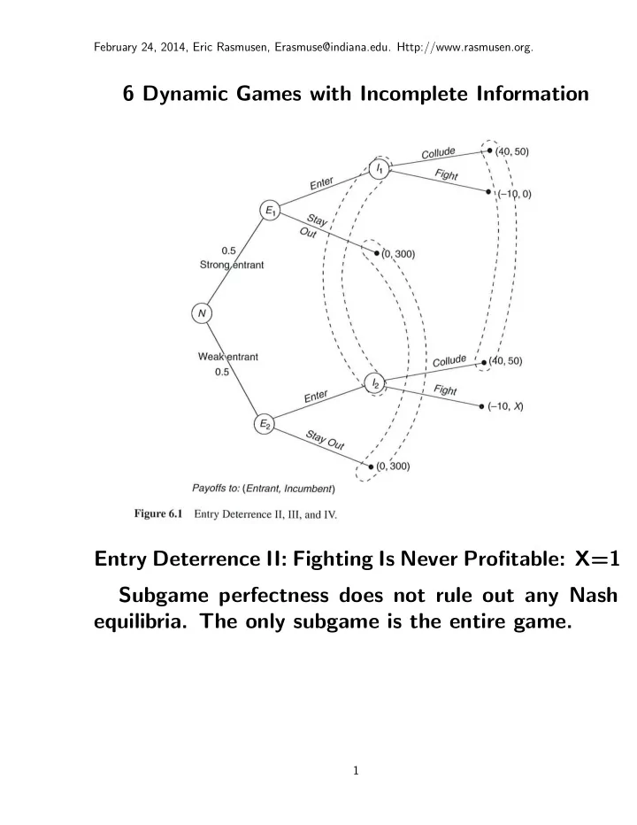
6 Dynamic Games with Incomplete Information Entry Deterrence II: Fighting Is Never Profitable: X=1 Subgame perfectness does not rule out any Nash

• equilibria. The only subgame is the entire game.

1

Trembling-Hand Perfectness Trembling-hand perfectness — Selten (1975) says a strategy that is to be part of an equilibrium must be

• ptimal for the player even if there is a small chance

that the other player’s hand will “tremble” : . The strategy profile s∗ is a trembling-hand perfect equilib- rium if for any ǫ there is a vector of positive numbers δ1, . . . , δn ∈ [0, 1] and a vector of completely mixed strategies σ1, . . . σn such that the perturbed game where every strategy is replaced by (1−δi)si +δiσi has a Nash equilibrium in which every strategy is within distance ǫ of s∗. This is hard to use, and undefined when games have continuous strategy spaces because it is hard to work with mixtures of a continuum).

2

Perfect Bayesian Equilibrium and Sequential Equilib- rium (Kreps & Wilson (1982)) The profile of beliefs and strategies is called an as- sessment. On the equilibrium path, all that the players need to update their beliefs are their priors and Bayes’ s Rule. Off the equilibrium path, this is not enough. Sup- pose that in equilibrium, the entrant always enters. If the entrant stays out, what is the incumbent to think about the probability the entrant is weak? Bayes’ s Rule does not help, because when Prob(data) = 0, which is the case for data such as Stay Out which is never observed in equilibrium, the posterior belief cannot be calculated using Bayes’ s Rule. Prob(Weak|Stay Out) = Prob(Stay Out|Weak)Prob(Weak) Prob(Stay Out) . (1) The posterior Prob(Weak|Stay Out) is undefined, because this requires dividing by zero.

3

A perfect bayesian equilibrium is a strategy profile s and a set of beliefs µ such that at each node of the game: (1) The strategies for the remainder of the game are Nash given the beliefs and strategies of the other players. (2) The beliefs at each information set are rational given the evidence appearing thus far in the game (meaning that they are based, if possible, on priors updated by Bayes’ s Rule, given the observed actions

• f the other players under the hypothesis that they

are in equilibrium). Kreps & Wilson (1982b) use this idea to form their equilibrium concept of sequential equilibrium, but they impose a third condition to restrict beliefs further: (3) The beliefs are the limit of a sequence of rational be- liefs, i.e., if (µ∗, s∗) is the equilibrium assessment, then some sequence of rational beliefs and completely mixed strategies converges to it: (µ∗, s∗) = Limn→∞(µn, sn) for some sequence (µn, sn) in {µ, s}.

4

Back to Entry Deterrence II A PBE for Entry Deterrence II : Entrant: Enter|Weak, Enter|Strong Incumbent: Collude Beliefs: Prob( Strong| Stay Out) = 0.4 There is no perfect bayesian equilibrium in which the entrant chooses Stay Out. Fight is a bad response even under the most opti- mistic possible belief, that the entrant is Weak with probability 1.

5

In Entry Deterrence III, assume X = 60, not X = 1. Fighting is now more profitable for the incumbent than collusion if the entrant is Weak. The first equilibrium we’ll examine uses passive conjectures— “posterior equals prior” for out-of-equilibrium beliefs, but could use ANY beliefs— it is completely robust.

6

A plausible pooling equilibrium for Entry Deter- rence III Entrant: Enter|Weak, Enter|Strong Incumbent: Collude, Out-of-equilibrium beliefs: Prob(Strong| Stay Out) = 0.5 In choosing whether to enter, the entrant must pre- dict the incumbent’s behavior. If the probability that the entrant is Weak is 0.5, the expected payoff to the incumbent from choosing Fight is 30 (= 0.5[0] + 0.5[60]), which is less than the payoff of 50 from Collude. The incumbent will collude, so the entrant enters. The entrant may know that the incumbent’s payoff is actually 60, but that is irrelevant to the incumbent’s behavior.

7

An implausible equilibrium for Entry Deterrence III Entrant: Stay Out|Weak, Stay Out|Strong Incumbent: Fight, Out-of-equilibrium beliefs: Prob(Strong|Enter) = 0.1 If the entrant were to deviate and enter, the incum- bent would calculate his payoff from fighting to be 54 (= 0.1[0] + 0.9[60]), which is greater than the Collude payoff of 50. The entrant would therefore stay out.

8

A conjectured separating equilibrium for Entry Deterrence III Entrant: Stay Out|Weak, Enter|Strong Incumbent: Collude This turns out not to be an equilibrium.

9

A Mixed-Strategy Equilibrium for Entry Deterrence III The prior for the probability that the entrant is strong is .5. In this game, the weak and the strong entrant both get the same payoff from entering. The strong entrant is strong only in the sense that the incumbent doesn’t want to fight him. Let the probability that the incumbent colludes be α. π(enter) = α(40) + (1 − α)(−10) = π(stay; out) = 0 Thus, α = .2. Let θ be the posterior probability that an entrant who enters is Strong. π(fight) = θ(0) + (1 − θ)(60) = π(collude) = 50 Thus, θ = 1/6. Let βs and βw be the probabilities with which the strong and weak entrants enter. We need θ = 1 6 = .5 · βs .5 · βw There are lots of values which satisfy this condition, e.g. βs = 1/6, βw = 1 or βs = 1/12, βw = 1/2 or βs = 1/10, βw = 6/10. The weak entrant is more likely to enter! The reason is that if the strong entrant were to enter with greater probability, the incumbent would want to Collude.

10

The PhD Admissions Game: A Separating Equilibrium A separating equilibrium for the PhD Admis- sions Game Student: Apply |Lover, Do Not Apply | Hater University: Admit

11

A pooling equilibrium for the PhD Admissions Game Student: Do Not Apply |Lover, Do Not Apply |Hater University: Reject, Out-of-equilibrium beliefs: Prob(Hater |Apply) = 0.9 (passive conjectures)

12

Passive Conjectures. Prob(Hater|Apply) = 0.9 This supports the pooling equilibrium. Complete Robustness. Prob(Hater|Apply) = m, 0 ≤ m ≤ 1 Under this approach, the equilibrium strategy pro- file must consist of responses that are best, given any and all out-of-equilibrium beliefs. Our equilibrium for Entry Deterrence II satisfied this requirement. Com- plete robustness rules out a pooling equilibrium in the PhD Admissions Game, because a belief like m = 0 makes accepting applicants a best response, in which case only the Lover will apply.

13

The Intuitive Criterion. Prob(Hater|Apply) = 0 Under the Intuitive Criterion of Cho & Kreps (1987), if there is a type of informed player who could not benefit from the out-of-equilibrium action no matter what beliefs were held by the uninformed player, the uninformed player’s belief must put zero probability

• n that type.

Here, the Hater could not benefit from applying un- der any possible beliefs of the university, so the uni- versity puts zero probability on an applicant being a Hater. This argument will not support the pooling equilibrium. An Ad Hoc Specification. Prob(Hater|Apply) = 1 Sometimes the modeller can justify beliefs by the circumstances of the particular game. Here, one could argue that anyone so foolish as to apply knowing that the university would reject them could not possibly have the good taste to love economics. This supports the pooling equilibrium also.

14

The Beer-Quiche Game of Cho & Kreps (1987). Player I is weak or strong and doesn’t want to duel. Player II wants to duel only if player I is weak. Player II does not know player I’s type, but he observes what player I has for breakfast. Weak players prefer quiche for breakast, strong players prefer beer. E1: Player I has beer. Player II doesn’t duel if beer, does duel if quiche. Out-of-equilibrium belief: a quiche- eating player I is weak with probability over 0.5. E2: Player I has quiche. Player II duel if beer doesn’t duel if quiche. Out-of-equilibrium belief: a beer-drinking player I is weak with probability over 0.5.

15

E2: Player I has quiche. Player II duel if beer doesn’t duel if quiche. Out-of-equilibrium belief: a beer-drinking player I is weak with probability over 0.5. Intuitive Criterion: player I could deviate to BEER by giving the following convincing speech, I am having beer for breakfast, which ought to convince you I am strong. The only con- ceivable benefit to me of breakfasting on beer comes if I am strong. I would never wish to have beer for breakfast if I were weak, but if I am strong and this message is convincing, then I benefit from having beer for breakfast.

16

Entry Deterrence IV: The Incumbent Benefits from His Own Ignorance Let X = 300. The entrant knows his type, but the incumbent does not. Equilibrium for Entry Deterrence IV Entrant: Stay Out |Weak, Stay Out |Strong Incumbent: Fight, Out-of-equilibrium beliefs: Prob(Strong|Enter) = 0.5 (passive conjectures)

17

There is no pure-strategy pooling equilibrium in which both types of entrant enter, because then the incumbent’s expected payoff from Fight would be 150 (= 0.5[0] + 0.5[300]), which is greater than the Collude payoff of 50. Nor is there a pure-strategy separating equilibrium. There exists a mixed-strategy equilibrium too.

18

Entry Deterrence V: Lack of Common Knowledge of Ignorance: Both the entrant and the incumbent know the payoff from (Enter, Fight), but the entrant does not know whether the incumbent knows. Entrant: Stay Out|Weak, Stay Out|Strong Incumbent: Fight|Nature said “Weak”, Collude|Nature said “Strong”, Fight |Nature said nothing, Out-of-equilibrium beliefs: Prob( Strong|Enter, Nature said nothing) = 0.5 (pas- sive conjectures)

19

Equilibrium for Entry Deterrence V Entrant: Stay Out|Weak, Stay Out|Strong Incumbent: Fight|Nature said “Weak”, Collude|Nature said “Strong”, Fight |Nature said nothing, Out-of- equilibrium beliefs: Prob( Strong|Enter, Nature said nothing) = 0.5 (passive conjectures) With probability 0.9, Nature has said nothing and the incumbent calculates his expected payoff from Fight to be 150, and with probability 0.05 (= 0.1[0.5]) Nature has told the incumbent that the entrant is weak and the payoff from Fight is 300. Even if the en- trant is strong and Nature tells this to the incumbent, the entrant would choose Stay Out, because he does not know that the incumbent knows, and his expected payoff from Enter would be −5 (= [0.9][−10] + 0.1[40]).

20

Kreps, Milgrom, Roberts, Wilson (1982) : The Gang

• f Four Model

One way to incorporate incomplete information would be to assume that with 30% probability Row is a player who blindly follows the strategy of Tit-for-Tat. If Column thinks he is playing against a Tit-for-Tat player, his optimal strategy is Silence until near the last period (how near depending on the parameters), and then Blame. If he were not certain of this, but the probabil- ity were high that he faced a Tit-for-Tat player, Row would choose that same strategy. But it turns out that even a small probability of a Tit-for-Tat player can make a big difference.

21

Theorem 6.1: The Gang of Four Theorem Consider a T-stage, repeated Prisoner’s Dilemma, with-

• ut discounting but with a probability γ of a Tit-for-

Tat player. In any perfect bayesian equilibrium, the number of stages in which either player chooses Blame is less than some number M that depends on γ but not on T. In equilibrium, Blame is played in the periods near

• T. Before that there is a period of mixing, and before

that they play Silence. The significance of the Gang of Four theorem is that while the players do resort to Blame as the last pe- riod approaches, the number of periods during which they Blame is independent of the total number of pe-

• riods. Suppose M = 2, 500. If T = 2, 500, there might

be Blame every period. But if T = 10, 000, there are 7,500 periods without a Blame move. For reasonable probabilities of the unusual type, the number of peri-

• ds of cooperation can be much larger.

Wilson has set up an entry deterrence model in which the incumbent fights entry (the equivalent of Silence above) up to seven periods from the end, al- though the probability the entrant is of the unusual type is only 0.008.

22

Gang of Four Intuition Column Silence Blame Silence 5,5

• 5,10

Row: Blame 10,-5 0,0 Payoffs to: (Row,Column) Consider what would happen in a 10,001-period PD with a probability of 0.01 that Row is playing the Grim Strategy. A best response for Column to a known Grim player is (Blame only in the last period, unless Row chooses Blame first, in which case respond with Blame). Column’s payoff will be 50,010 (= (10,000)(5) + 10). Blame Always would just yield 10 as a payoff. Suppose instead that if Row is not Grim, he will choose Blame every period. The outcome will be (Blame, Silence) in the first period and (Blame, Blame) thereafter, for a payoff to Column of −5(= −5 + (10, 000)(0)). If the probabilities of the two

• utcomes are 0.01 and 0.99, Column’s expected pay-
• ff is 495.15.

If instead Row follows a strategy of (Blame every period), his expected payoff is just 0.1 (= 0.01(10) + 0.99(0)).

23

Column Silence Blame Silence 5,5

• 5,10

Row: Blame 10,-5 0,0 Payoffs to: (Row,Column) The aggressive strategy is not Row’s best response to Column’s strategy. A better response is for Row to choose Silence until the second-to-last period, and then Blame. Row’s payoff would rise from 10 to (9,999)(5) + 10. Given that Column is cooperating in the early peri-

• ds, Row will cooperate also. Still not Nash, but we

see why Column chooses Silence in the first period.

24

Theorem 6.2: The Incomplete Information Folk The-

• rem(Fudenberg & Maskin [1986] p. 547)

For any two-person repeated game without discount- ing, the modeller can choose a form of irrationality so that for any probability ǫ > 0 there is some finite num- ber of repetitions such that with probability (1 − ǫ) a player is rational and the average payoffs in some se- quential equilibrium are closer than ǫ to any desired payoffs greater than the minimax payoffs.

25

THE AXELROD TOURNAMENT: Contestants sub- mitted strategies for a 200-repetition Prisoner’s Dilemma . Since the strategies could not be updated during play, players could precommit, but the strategies could be as complicated as they wished. Strategies were submitted in the form of computer

• programs. In Axelrod’s first tournament, 14 programs

were submitted as entries. Every program played ev- ery other program, and the winner was the one with the greatest sum of payoffs over all the plays. The winner was Anatol Rapoport, whose strategy was Tit- for-Tat. What strategy could have beat Rapoport and all the others? After the results of the first tournament were an- nounced, Axelrod ran a second tournament, adding a probability θ = 0.00346 that the game would end each round so as to avoid the Chainstore Paradox. The win- ner among the 62 entrants was again Anatol Rapoport with Tit-for-Tat.

26

Before choosing his tournament strategy, Rapoport had written an entire book on The Prisoner’s Dilemma in analysis, experiment, and simulation. Why did he choose such a simple strategy as Tit- for-Tat? Tit-for-Tat has three strong points.

• 1. It never initiates blaming (niceness);
• 2. It retaliates instantly against blaming (provocabil-

ity);

• 3. It forgives someone who plays Blame but then goes

back to cooperating (it is forgiving). Tit-for-Tat never beats any other strategy in a one-

• n-one contest.

In an elimination tournament, Tit- for- Tat would be eliminated early, because it scores high payoffs but never the highest payoff. In a game in which players occasionally blamed be- cause of trembles, two Tit-for-Tat players facing each

• ther would do very badly.

27

“Reputation Acquisition in Debt Markets” JPE, 1989 Douglas Diamond (1989) explains why old firms are less likely than young firms to default on debt. The three types of risk-neutral firms, R, S, and RS, are “born” at time zero and borrow to finance projects at the start of each of T periods. Type RS firms can choose independently risky projects with negative expected values or safe projects with low but positive expected values. Although the risky projects are worse in expecta- tion, if they are successful the return is much higher than from safe projects. Type R firms can only choose risky projects, and type S firms only safe projects. At the end of each period the projects bring in their profits and loans are repaid, after which new loans and projects are chosen for the next period. Lenders cannot see which project is chosen or a firm’s current profits, but they can seize the firm’s assets if a loan is not repaid, which always happens if the risky project was chosen and turned out unsuccessfully.

28

The equilibrium path has three parts. The RS firms start by choosing risky projects. Their downside risk is limited by bankruptcy, but if the project is suc- cessful the firm keeps large profits after repaying the loan. Over time, the number of firms with access to the risky project (the RS’s and R’s) diminishes through bankruptcy, while the number of S’s remains unchanged. Lenders can therefore maintain zero profits while lowering their interest rates. When the interest rate falls, the value of a stream of safe investment profits minus interest payments rises relative to the expected value of the few periods of risky returns minus interest payments before bankruptcy.

29

After the interest rate has fallen enough, the second phase of the game begins when the RS firms switch to safe projects, at t1. Only the tiny and diminish- ing group of type R firms continue to choose risky projects. Since the lenders know that the RS firms switch, the interest rate falls sharply at t1. A firm that is older is less likely to be a type R, so it is charged a lower interest rate.

30

Towards T, the value of future profits from safe projects declines and the RS’s are again tempted to choose risky projects. Between t2 and t3, the RS’s follow a mixed strategy, an increasing number choosing risky projects. The interest rate rises as a result. At t3, the interest rate is high enough and the end

• f the game is close enough that the RS’s revert to

the pure strategy of choosing risky projects. The in- terest rate then falls as the number of RS’s diminishes because of failed risky projects.

31

Why three types of firms, not two? Types S and RS are clearly needed, but why type R? The little extra detail in the game description al- lows simplification of the equilibrium, because with three types bankruptcy is never out-of-equilibrium be- haviour, since the failing firm might be a type R. Bayes’s Rule can therefore always be applied, elmi- nating the problem of ruling out peculiar beliefs and absurd perfect bayesian equilibria. This is a Gang of Four model but differs from pre- vious examples in an important respect: the Diamond model is not stationary, and as time progresses, some firms of types R and RS go bankrupt, which changes the lenders’ payoff functions. Thus, it is not a re- peated game.

32