6. Direct Volume Rendering Directly get a 3D representation of the - - PDF document

Visualization, Summer Term 03 VIS, University of Stuttgart

1

• 6. Direct Volume Rendering
• Directly get a 3D representation of the volume

data

• The data is considered to represent a semi-

transparent light-emitting medium

• Also gaseous phenomena can be simulated
• Approaches are based on the laws of physics

(emission, absorption, scattering)

• The volume data is used as a whole

(look inside, see all interior structures)

Visualization, Summer Term 03 VIS, University of Stuttgart

2

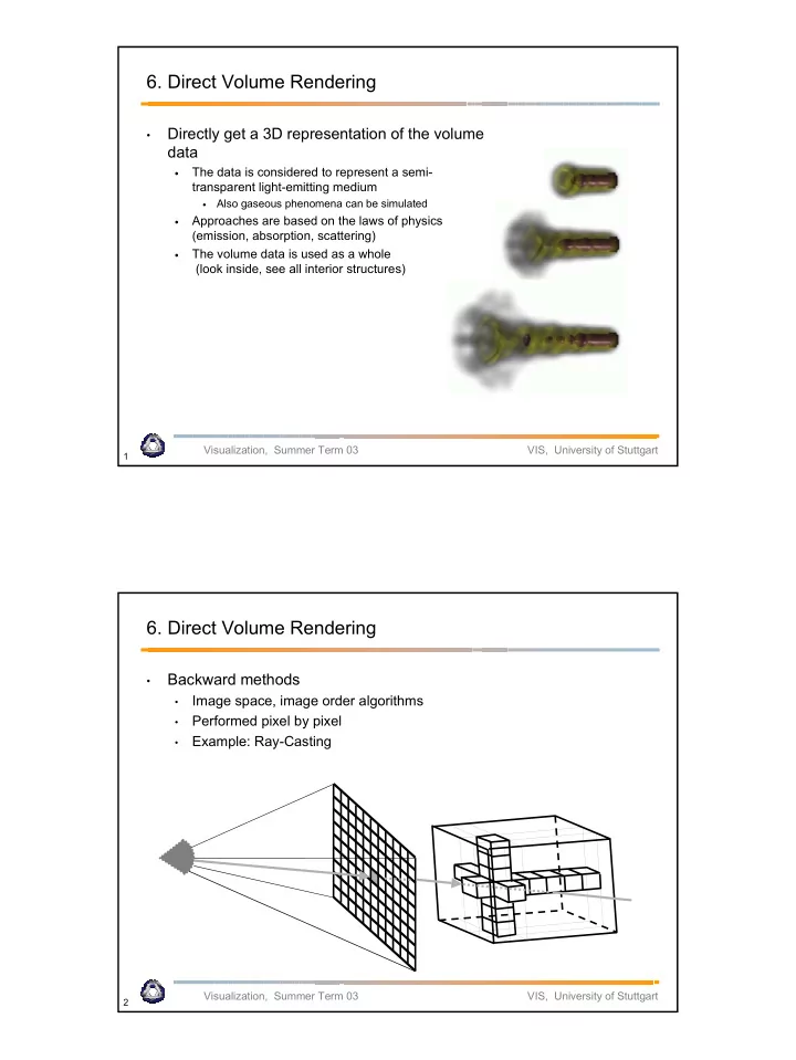
• 6. Direct Volume Rendering
• Backward methods
• Image space, image order algorithms
• Performed pixel by pixel
• Example: Ray-Casting

Visualization, Summer Term 03 VIS, University of Stuttgart

3

• 6. Direct Volume Rendering
• Forward Methods
• Object space, object order algorithm
• Cell projection
• Performed voxel by voxel
• Examples: Slicing, shear-warp, splatting

Visualization, Summer Term 03 VIS, University of Stuttgart

4

6.1. Ray Casting

• Similar to ray tracing in surface-based computer graphics
• In volume rendering we only deal with primary rays; hence: ray-casting
• Natural image-order technique
• As opposed to surface graphics - how do we calculate the ray/surface

intersection ?

Visualization, Summer Term 03 VIS, University of Stuttgart

5

6.1. Ray Casting

• Since we have no surfaces - we need to carefully step through the volume
• A ray is cast into the volume, sampling the volume at certain intervals
• Sampling intervals are usually equidistant, but don’t have to be (e.g.

importance sampling)

• At each sampling location, a sample is interpolated / reconstructed from the

voxel grid

• Popular filters are: nearest neighbor (box), trilinear, or more sophisticated

(Gaussian, cubic spline)

Visualization, Summer Term 03 VIS, University of Stuttgart

6

6.1. Ray Casting

• Volumetric ray integration:
• Tracing of rays
• Accumulation of color and opacity along ray: compositing

color

• bject (color, opacity)

1.0

Visualization, Summer Term 03 VIS, University of Stuttgart

7

6.1. Ray Casting

color

• pacity

1.0 interpolation kernel

• bject (color, opacity)

volumetric compositing

Visualization, Summer Term 03 VIS, University of Stuttgart

8

6.1. Ray Casting

color c = αsc s (1 - α) + c

• pacity α = α s (1 - α) + α

1.0

• bject (color, opacity)

volumetric compositing 1.0 interpolation kernel

Visualization, Summer Term 03 VIS, University of Stuttgart

9

6.1. Ray Casting

color

• pacity

1.0

• bject (color, opacity)

volumetric compositing

Visualization, Summer Term 03 VIS, University of Stuttgart

10

6.1. Ray Casting

color

• pacity

1.0

• bject (color, opacity)

volumetric compositing

Visualization, Summer Term 03 VIS, University of Stuttgart

11

6.1. Ray Casting

color

• pacity

1.0

• bject (color, opacity)

volumetric compositing

Visualization, Summer Term 03 VIS, University of Stuttgart

12

6.1. Ray Casting

color

• pacity

1.0

• bject (color, opacity)

volumetric compositing

Visualization, Summer Term 03 VIS, University of Stuttgart

13

6.1. Ray Casting

color

• pacity
• bject (color, opacity)

volumetric compositing

Visualization, Summer Term 03 VIS, University of Stuttgart

14

6.1. Ray Casting

• How is color and opacity at each integration step determined?
• Opacity and (emissive) color in each cell according to classification
• Additional color due to external lighting:

according to volumetric shading (e.g. Blinn-Phong)

• No shadowing, no secondary effects

Visualization, Summer Term 03 VIS, University of Stuttgart

15

• Compositing of semi-transparent voxels
• Physical model: emissive gas with absorption
• Approximation: density-emitter-model (no scattering)
• Over operator [Porter & Duff 1984]
• Cout = Cin (1 - α) + C α = C~ over Cin

with premultiplied Color C~ = C α

6.1. Ray Casting

Cin Cout C, α CN

• ut

Ci, αi C0

in

back-to-front strategy (BTF) Ci

in = Ci-1

• ut

Ci

• ut = Ci

in(1-αi)+ Ciαi

= (Ci-1

in(1-αi-1)+ Ci-1 αi-1) (1-αi)+ Ci αi

= ∑ i=1,n Ci αi Πj=i+1,n (1-αj)

Visualization, Summer Term 03 VIS, University of Stuttgart

16

6.1. Ray Casting

• Compositing of semi-transparent voxels (cont.)
• Variation of previous approach for front-to-back strategy (FTB)
• Cout = Cin +(1 - αin) αC
• αout = αin +(1 - αin) α
• Needs to maintain α !

Cin, αin Cout , αout C, α

Visualization, Summer Term 03 VIS, University of Stuttgart

17

• Traversal strategies
• Front-to-back (most often used in ray casting)
• Back-to-front (e.g., in texture-based volume rendering)
• Discrete (Bresenham) or continuous (DDA) traversal of cells

6.1. Ray Casting

Visualization, Summer Term 03 VIS, University of Stuttgart

18

6.2. Acceleration Techniques for Ray Casting

• Problem: ray casting is time consuming
• Idea:
• Neglect „irrelevant“ information to accelerate the rendering process
• Exploit coherence
• Early-ray termination
• Idea: colors from faraway regions do

not contribute if accumulated opacity is to high

• Stop traversal if contribution of sample

becomes irrelevant

• User-set opacity level for termination
• Front-to-back compositing

Visualization, Summer Term 03 VIS, University of Stuttgart

19

6.2. Acceleration Techniques for Ray Casting

• Space leaping
• Skip empty cells
• Homogeneity-acceleration
• Approximate homogeneous regions

with fewer sample points

• Approaches:
• Hierarchical spatial data structure
• Bounding boxes around objects
• Adaptive ray traversal
• Proximity clouds

Visualization, Summer Term 03 VIS, University of Stuttgart

20

6.2. Acceleration Techniques for Ray Casting

• Hierarchical spatial data structure
• Octree
• Mean value and variance stored in nodes of
• ctree
• Flat Pyramid: store octree level in “empty”

voxels

• Bounding boxes around objects
• Polygon assisted ray casting (PARC)

Visualization, Summer Term 03 VIS, University of Stuttgart

21

6.2. Acceleration Techniques for Ray Casting

• Adaptive ray traversal
• Different „velocities“ for traversal
• Different distance between samples
• Based on vicinity flag
• Layer of „vicinity voxels“ around non-

transparent parts of the volume

Visualization, Summer Term 03 VIS, University of Stuttgart

22

6.2. Acceleration Techniques for Ray Casting

• Proximity clouds
• Extension of vicinity voxels
• Store distance to closest „object“ in voxels
• Allows large integration steps

Visualization, Summer Term 03 VIS, University of Stuttgart

23

6.2. Acceleration Techniques for Ray Casting

• Exploiting temporal coherence in volume

animations

• C-buffer (Coordinates buffer)
• Store coordinates of first opaque voxel
• Removing potentially hidden voxels
• Or adding potentially visible voxels
• Criterion: change of position on image plane

Visualization, Summer Term 03 VIS, University of Stuttgart

24

6.2. Acceleration Techniques for Ray Casting

• Template-based volume viewing [Yagel 1991]
• Ray template stores traversal (steps) through volume
• Generate template by 3D DDA for parallel rays (orthographic projection)
• Starting ray templates at pixel positions leads to sampling artefacts
• Start template ray from base plane parallel to volume orientation
• Warp image on base plane to view plane

base plane template view plane

Visualization, Summer Term 03 VIS, University of Stuttgart

25

6.2. Acceleration Techniques for Ray Casting

• Adaptive screen sampling [Levoy 1990]
• Rays are emitted from a subset of pixels (on image plane)
• Missing values are interpolated
• In areas of high value gradient additional rays are traced

Visualization, Summer Term 03 VIS, University of Stuttgart

26

6.3. Texture-Based Volume Rendering

• Object-space approach
• Based on graphics hardware:
• Rasterization
• Texturing
• Blending
• Proxy geometry because there are no volumetric primitives in graphics

hardware

• Slices through the volume

Visualization, Summer Term 03 VIS, University of Stuttgart

27

6.3. Texture-Based Volume Rendering

• Slice-based rendering

color

• pacity
• bject (color, opacity)

Similar to ray casting with simultaneous rays

Visualization, Summer Term 03 VIS, University of Stuttgart

28

6.3. Texture-Based Volume Rendering

pixels vertices primitives fragments scene description geometry processing geometry processing rasterization rasterization fragment

• perations

fragment

• perations

rendering pipeline

Visualization, Summer Term 03 VIS, University of Stuttgart

29

6.3. Texture-Based Volume Rendering

• Proxy geometry
• Stack of texture-mapped slices
• Generate fragments
• Most often back-to-front traversal

Visualization, Summer Term 03 VIS, University of Stuttgart

30

6.3. Texture-Based Volume Rendering

• 2D textured slices
• Object-aligned slices
• Three stacks of 2D textures
• Bilinear interpolation

Visualization, Summer Term 03 VIS, University of Stuttgart

31

6.3. Texture-Based Volume Rendering

• 3D textured slices
• View-aligned slices
• Single 3D texture
• Trilinear interpolation

Visualization, Summer Term 03 VIS, University of Stuttgart

32

6.3. Texture-Based Volume Rendering

texturing (trilinear interpolation) texturing (trilinear interpolation) compositing (blending) compositing (blending) texturing (bilinear interpolation) texturing (bilinear interpolation) compositing (blending) compositing (blending)

2D textures axis-aligned 3D texture view-aligned

Visualization, Summer Term 03 VIS, University of Stuttgart

33

6.3. Texture-Based Volume Rendering

• Stack of 2D textures:
• Works on older graphics hardware which does not support 3D textures
• Only bilinear interpolation within slices, no trilinear interpolation
• > fast
• > problems with image quality
• Euclidean distance between slices along a light ray depends on viewing

parameters

• > sampling distance depends on viewing direction
• > apparent brightness changes if opacity is not corrected
• Artifacts when stack is viewed close to 45 degrees

Visualization, Summer Term 03 VIS, University of Stuttgart

34

6.3. Texture-Based Volume Rendering

• Change of brightness in 2D texture-based rendering

Visualization, Summer Term 03 VIS, University of Stuttgart

35

6.3. Texture-Based Volume Rendering

• Artifacts when stack is viewed close to 45 degrees

Visualization, Summer Term 03 VIS, University of Stuttgart

36

6.3. Texture-Based Volume Rendering

• 3D texture:
• Needs support for 3D textures
• Trilinear interpolation within volume
• > slower
• > good image quality
• Constant Euclidean distance between slices along a light ray
• No artifacts due to inappropriate viewing angles

Visualization, Summer Term 03 VIS, University of Stuttgart

37

6.3. Texture-Based Volume Rendering

• Render components
• Data setup
• Volume data representation
• Transfer function representation
• Data download
• Volume textures
• Transfer function tables
• Per-volume setup (once per frame)
• Blending mode configuration
• Texture unit configuration (3D)
• (Fragment shader configuration)
• Per-slice setup
• Texture unit configuration (2D)
• Generate fragments
• Proxy geometry rendering

Visualization, Summer Term 03 VIS, University of Stuttgart

38

6.3. Texture-Based Volume Rendering

• Representation of volume data by textures
• Stack of 2D textures
• 3D texture
• Typical choices for texture format:
• Intensity
• Scalar data, post-classification only with special
• OpenGL extension GL_TEXTURE_COLOR_TABLE_SGI
• dependent texture lookups (pixel shader)
• Luminance and alpha
• Pre-classified (pre-shaded) gray-scale volume rendering
• Transfer function is already applied to scalar data
• Change of transfer function requires complete redefinition of texture data
• RGBA
• Pre-classified (pre-shaded) colored volume rendering
• Transfer function is already applied to scalar data

Visualization, Summer Term 03 VIS, University of Stuttgart

39

6.3. Texture-Based Volume Rendering

• Typical choices for texture format (cont.):
• Paletted texture
• Index into color and opacity table (= palette)
• Index size = byte
• Index is identical to scalar value
• Pre-classified (pre-shaded) colored volume rendering
• Transfer function applied to scalar data during runtime
• Simple and fast change of transfer functions
• OpenGL code for paletted 3D texture

glTexImage3D ( GL_TEXURE_3D, 0, GL_COLOR_INDEX8_EXT, size_x, size_y, GL_COLOR_INDEX, GL_UNSIGNED_BYTE, voldata);

Visualization, Summer Term 03 VIS, University of Stuttgart

40

6.3. Texture-Based Volume Rendering

• Representation of transfer function:
• For paletted texture only
• 1D transfer function texture = lookup table
• OpenGL code

glColorTableEXT (GL_SHARED_TEXTURE_PALETTE_EXT, GL_RGBA8, 256*4, GL_RGBA, GL_UNSIGNED_BYTE, palette);

• OpenGL extensions required

Visualization, Summer Term 03 VIS, University of Stuttgart

41

6.3. Texture-Based Volume Rendering

• Compositing:
• Works on fragments
• Per-fragment operations
• After rasterization
• Blending of fragments via over operator
• OpenGL code for over operator

glEnable (GL_BLEND); glBlendFunc (GL_SRC_ALPHA, GL_ONE_MINUS_SRC_ALPHA);

• Generate fragments:
• Render proxy geometry
• Slice
• Simple implementation: quadrilateral
• More sophisticated: triangulated intersection surface between slice plane

and boundary of the volume data set

Visualization, Summer Term 03 VIS, University of Stuttgart

42

6.3. Texture-Based Volume Rendering

• Advantages of texture-based rendering:
• Supported by consumer graphics hardware
• Fast for moderately sized data sets
• Interactive explorations
• Surface-based and volumetric representations can easily be combined
• > mixture with opaque geometries
• Disadvantages:
• Limited by texture memory
• > Solution: bricking at the cost of additional texture downloads to the

graphics board

• Brute force: complete volume is represented by slices
• No acceleration techniques like early-ray termination or space leaping
• Rasterization speed and memory access can be problematic

Visualization, Summer Term 03 VIS, University of Stuttgart

43

6.3. Texture-Based Volume Rendering

• Outlook on more advanced texture-based volume rendering

techniques:

• Exploit quite flexible per-fragment operations on modern GPUs (nVidia

GeForce 3/4 or ATI Radeon 8500)

• Post-classification (post-shading) possible
• So-called pre-integration for very high-quality rendering
• Decompression of compressed volumetric data sets on GPU to save

texture memory

Visualization, Summer Term 03 VIS, University of Stuttgart

44

6.4. Shear-Warp Factorization

• Object-space method
• Slice-based technique
• Fast object-order rendering
• Accelerated volume visualization via

shear-warp factorization [Lacroute & Levoy 1994]

• Software-based implementation

Visualization, Summer Term 03 VIS, University of Stuttgart

45

6.4. Shear-Warp Factorization

• General goal: make viewing rays parallel to each other and

perpendicular to the image

• This is achieved by a simple shear
• Parallel projection (orthographic camera) is assumed
• Extension for perspective projection possible

shear warp

Visualization, Summer Term 03 VIS, University of Stuttgart

46

6.4. Shear-Warp Factorization

• Algorithm:
• Shear along the volume slices
• Projection and compositing to get intermediate image
• Warping transformation of intermediate image to get correct result

view rays slices view plane shear transformation: warp projection

Visualization, Summer Term 03 VIS, University of Stuttgart

47

6.4. Shear-Warp Factorization

• For one scan line

Visualization, Summer Term 03 VIS, University of Stuttgart

48

6.4. Shear-Warp Factorization

• Mathematical description of the shear-warp factorization
• Splitting the viewing transformation into separate parts
• Mview

= general viewing matrix

• P

= permutation matrix: transposes the coordinate system in

• rder to make the z-axis the principal viewing axis
• S

= transforms volume into sheared object space

• Mwarp

= warps sheared object coordinates into image coordinates

• Needs 3 stacks of the volume along 3 principal axes

warp view

M S P M ⋅ ⋅ =

Visualization, Summer Term 03 VIS, University of Stuttgart

49

6.4. Shear-Warp Factorization

• Shear for parallel and perspective projections

              = 1 1 1 1

par y x

s s S               ′ ′ ′ = 1 1 1 1

persp w y x

s s s S

shear & scale warp shear perpendicular to z-axis shear and scale perspective projection

Visualization, Summer Term 03 VIS, University of Stuttgart

50

6.4. Shear-Warp Factorization

• Algorithm (detailed):
• Transform volume to sheared object space by translation and resampling
• Project volume into 2D intermediate image in sheared object space
• Composite resampled slices front-to-back
• Transform intermediate image to image space using 2D warping
• In a nutshell:
• Shear (3D)
• Project (3D 2D)
• Warp (2D)

Visualization, Summer Term 03 VIS, University of Stuttgart

51

6.4. Shear-Warp Factorization

• Three properties
• Scan lines of pixels in the intermediate image are parallel to scan lines of

voxels in the volume data

• All voxels in a given voxel slice are scaled by the same factor
• Parallel projections only:

Every voxel slice has the same scale factor

• Scale factor for parallel projections
• This factor can be chosen arbitrarily
• Choose a unity scale factor so that for a given voxel scan line there is a
• ne-to-one mapping between voxels and intermediate image pixels

Visualization, Summer Term 03 VIS, University of Stuttgart

52

6.4. Shear-Warp Factorization

• Highly optimized algorithm for
• Parallel projection and
• Fixed opacity transfer function
• Optimization of volume data (voxel scan lines)
• Run-length encoding of voxel scan lines
• Skip runs of transparent voxels
• Transparency and opaqueness determined by user-defined opacity

threshold

• Optimization in intermediate image:
• Skip opaque pixels in intermediate image (analogously to early-ray

termination)

• Store (in each pixel) offset to

next non-opaque pixel

Visualization, Summer Term 03 VIS, University of Stuttgart

53

6.4. Shear-Warp Factorization

• Combining both ideas:
• First property (parallel scan lines for pixels and voxels):

Voxel scan lines in sheared volume are aligned with pixel scan lines in intermediate

• Both can be traversed in scan line order simultaneously

Visualization, Summer Term 03 VIS, University of Stuttgart

54

6.4. Shear-Warp Factorization

• Coherence in voxel space:
• Each slice of the volume is only translated
• Fixed weights for bilinear interpolation within voxel slices
• Computation of weights only once per frame
• Final warping:
• Works on composited intermediate image
• Warp: affine image warper with bilinear filter
• Often done in hardware:

render a quadrilateral with intermediate 2D image being attached as 2D texture

Visualization, Summer Term 03 VIS, University of Stuttgart

55

6.4. Shear-Warp Factorization

• Parallel projection:
• Efficient reconstruction
• Lookup table for shading
• Lookup table for opacity correction (thickness)
• Three RLE of the actual volume (in x, y, z)
• Perspective projection:
• Similar to parallel projection
• Difference: voxels need to be scaled
• Hence more than two voxel scan lines needed for one image scan line

Visualization, Summer Term 03 VIS, University of Stuttgart

56

6.5. Splatting

• Splatting [Westover 1990]
• Object-order method
• Original method: fast, poor quality
• Many improvements since then

Visualization, Summer Term 03 VIS, University of Stuttgart

57

6.5. Splatting

• Project each sample (voxel) from the volume into the image plane

image splat

Visualization, Summer Term 03 VIS, University of Stuttgart

58

6.5. Splatting

Visualization, Summer Term 03 VIS, University of Stuttgart

59

6.5. Splatting

• Ideally we would reconstruct the continuous volume (cloud) using the

interpolation kernel w (spherically symmetric):

• Analytic integral along a ray r for intensity (emission):
• Rewrite:

∑

− =

k k k r

v f v v w v f ) ( ) ( ) (

( ) ( )

∫∑ ∫

− + = + =

k k k r

dr v f v r p w dr r p f p I ) ( ) (

( ) ( )

∑ ∫

− + ⋅ =

k k k

dr v r p w v f p I ) (

splatting kernel (= “splat”)

Visualization, Summer Term 03 VIS, University of Stuttgart

60

• Discretization via 2D splats

from the original 3D kernel

• The 3D rotationally symmetric filter kernel is integrated to produce a

2D filter kernel

6.5. Splatting

( )dz

z y x w y x

∫

= , , ) , ( Splat

3D filter kernel Integrate along one dimension 2D filter kernel

Visualization, Summer Term 03 VIS, University of Stuttgart

61

6.5. Splatting

• Draw each voxel as a cloud of points (footprint) that spreads the voxel

contribution across multiple pixels

• Footprint: splatted (integrated) kernel
• Approximate the 3D kernel h(x,y,z) extent by a sphere

Visualization, Summer Term 03 VIS, University of Stuttgart

62

6.5. Splatting

• Larger footprint increases blurring and used for

high pixel-to-voxel ratio

• Footprint geometry
• Orthographic projection: footprint is independent of

the view point

• Perspective projection: footprint is elliptical
• Pre-integration of footprint
• For perspective projection: additional

computation of the orientation of the ellipse

Visualization, Summer Term 03 VIS, University of Stuttgart

63

6.5. Splatting

• The choice of kernel can affect the

quality of the image

• Examples are cone, Gaussian,

sinc, and bilinear function

• Effects of kernel function

1D integration of 3D Gaussian is a 2D Gaussian

Visualization, Summer Term 03 VIS, University of Stuttgart

64

6.5. Splatting

• Volume = field of 3D interpolation kernels
• One kernel at each grid voxel
• Each kernel leaves a 2D footprint on screen
• Weighted footprints accumulate into image

voxel kernels screen footprints = splats screen

Visualization, Summer Term 03 VIS, University of Stuttgart

65

6.5. Splatting

• Volume = field of 3D interpolation kernels
• One kernel at each grid voxel
• Each kernel leaves a 2D footprint on screen
• Weighted footprints accumulate into image

voxel kernels screen footprints = splats screen

Visualization, Summer Term 03 VIS, University of Stuttgart

66

6.5. Splatting

• Volume = field of 3D interpolation kernels
• One kernel at each grid voxel
• Each kernel leaves a 2D footprint on screen
• Weighted footprints accumulate into image

voxel kernels screen footprints = splats screen

Visualization, Summer Term 03 VIS, University of Stuttgart

67

6.5. Splatting

• Voxel kernels are added within sheets
• Sheets are composited front-to-back
• Sheets = volume slices most perpendicular to the image plane

(analogously to stack of slices)

image plane at 70° image plane at 30° volume slices x y z volume slices

Visualization, Summer Term 03 VIS, University of Stuttgart

68

6.5. Splatting

• Core algorithm for splatting
• Volume
• Represented by voxels
• Slicing
• Image plane:
• Sheet buffer
• Compositing buffer

sheet buffer compositing buffer volume slices image plane

Visualization, Summer Term 03 VIS, University of Stuttgart

69

6.5. Splatting

• Add voxel kernels within first sheet

sheet buffer compositing buffer image plane volume slices

Visualization, Summer Term 03 VIS, University of Stuttgart

70

6.5. Splatting

• Transfer to compositing buffer

sheet buffer compositing buffer image plane volume slices

Visualization, Summer Term 03 VIS, University of Stuttgart

71

6.5. Splatting

• Add voxel kernels within second sheet

sheet buffer compositing buffer image plane volume slices

Visualization, Summer Term 03 VIS, University of Stuttgart

72

6.5. Splatting

• Composite sheet with compositing buffer

sheet buffer compositing buffer image plane volume slices

Visualization, Summer Term 03 VIS, University of Stuttgart

73

6.5. Splatting

• Add voxel kernels within third sheet

volume slices sheet buffer compositing buffer image plane

Visualization, Summer Term 03 VIS, University of Stuttgart

74

6.5. Splatting

• Composite sheet with compositing buffer

sheet buffer compositing buffer image plane volume slices

Visualization, Summer Term 03 VIS, University of Stuttgart

75

6.5. Splatting

• Inaccurate compositing
• Problems when splats overlap
• Incorrect mixture of
• Integration (3D kernel to 2D splat)

and

• Compositing

problematic

Visualization, Summer Term 03 VIS, University of Stuttgart

76

6.5. Splatting

• Advantages:
• Footprints can be pre-integrated
• Quite fast: voxel interpolation is in 2D on screen
• Simple static parallel decomposition
• Acceleration approach: only relevant voxels must be projected
• Disadvantages:
• Blurry images for zoomed views
• High fill-rate for zoomed splats
• Reconstruction and integration to be performed on a per-splat basis
• Dilemma when splats overlap

Visualization, Summer Term 03 VIS, University of Stuttgart

77

6.5. Splatting

• Simple extension to volume data without

grids

• Scattered data with kernels
• Example: SPH (smooth particle

hydrodynamics)

• Needs sorting of sample points

Visualization, Summer Term 03 VIS, University of Stuttgart

78

6.6. Equation of Transfer for Light

• Goal: physical model for volume rendering
• Emission-absorption model
• Density-emitter model [Sabella 1988]
• More general approach:
• Linear transport theory
• Equation of transfer for radiation
• Basis for all rendering methods
• Important aspects:
• Absorption
• Emission
• Scattering
• Participating medium

Visualization, Summer Term 03 VIS, University of Stuttgart

79

6.6. Equation of Transfer for Light

• The Grand Scheme

Geometric Optics No Medium No Scattering

Equation of Transfer Volume Rend Equation Rendering Equation Radiosity Equation

Visualization, Summer Term 03 VIS, University of Stuttgart

80

6.6. Equation of Transfer for Light

• Assumptions:
• Based on a physical model for radiation
• Geometrical optics
• Neglect:
• Diffraction
• Interference
• Wave-character
• Polarization
• Interaction of light with matter at the macroscopic scale
• Describes the changes of specific intensity due to absorption, emission,

and scattering

• Based on energy conservation
• Expressed by equation of transfer

Visualization, Summer Term 03 VIS, University of Stuttgart

81

6.6. Equation of Transfer for Light

• Basic quantity of light: radiance I
• Sometimes called specific intensity

dt d d dA I E ν θ ν δ Ω = cos ) , , ( n x

radiative energy radiance position direction dΩ dA θ n frequency projected area element solid angle time

Visualization, Summer Term 03 VIS, University of Stuttgart

82

6.6. Equation of Transfer for Light

• Contributions to radiation at a single position:
• Absorption
• Emission
• Scattering

Visualization, Summer Term 03 VIS, University of Stuttgart

83

6.6. Equation of Transfer for Light

• Absorption
• Total absorption coefficient or total extinction coefficient χ(x,n,ν)
• Loss of radiative energy through a cylindrical volume element:
• 1/ χ is called mean free path

dΩ ds dΩ’ dI’ dI

dt d d dA ds I E ν ν ν χ δ Ω = ) , , ( ) , , (

(ab)

n x n x

Visualization, Summer Term 03 VIS, University of Stuttgart

84

6.6. Equation of Transfer for Light

• Total absorption coefficient consists of:
• True absorption coefficient κ(x,n,ν)
• Scattering coefficient σ(x,n,ν)

scattering out of solid angle dΩ dΩ ds dΩ’ dI’ dI removal of radiative energy by true absorption (conversion to thermal energy)

σ κ χ + =

Visualization, Summer Term 03 VIS, University of Stuttgart

85

6.6. Equation of Transfer for Light

• Emission
• Emission coefficient η(x,n,ν)
• Emission of radiative energy within a cylindrical volume element:
• Consists of two parts:
• Thermal part or source term q(x,n,ν)
• Scattering part j(x,n,ν)

dt d d dA ds E ν ν η δ Ω = ) , , (

(em)

n x j q + = η

Visualization, Summer Term 03 VIS, University of Stuttgart

86

6.6. Equation of Transfer for Light

• Scattering
• Described by phase function p(x,n,n‘,ν,ν‘)
• Elastic scattering:
• No change of frequency
• p(x,n,n‘)

' ' ) ' , , ' , , ( 4 1

(scat)

ν ν ν π ν σ δ d d p dt d d dA ds I E Ω ⋅ Ω = n n x

Visualization, Summer Term 03 VIS, University of Stuttgart

87

6.6. Equation of Transfer for Light

participating medium volume scattering surface scattering interface between materials

Visualization, Summer Term 03 VIS, University of Stuttgart

88

6.6. Equation of Transfer for Light

• Conservation of energy: difference of radiative energy along light ray

must be equal to difference between effects of emission and absorption ⇒

{ } { }

dt d d dA ds I dt d d dA d I I ν ν η ν ν χ ν ν ν Ω + − = Ω + − ) , , ( ) , , ( ) , , ( ) , , ( ) , , ( n x n x n x n x x n x η χ + − = ∇

• I

I n

time-independent equation of transfer

Visualization, Summer Term 03 VIS, University of Stuttgart

89

6.6. Equation of Transfer for Light

• Note: scattering part contains I
• Writing out the equation of transfer:
• Without frequency-dependency and without inelastic scattering:

( )

∫∫

Ω + + + − = ∇

• '

' ) ' , ' , ( ) , ' , , ' , ( ) ' , ' , ( 4 1 ν ν ν ν ν σ π σ κ d d I p q I I n x n n x n x n

( )

∫

Ω + + + − = ∇

• '

) ' , ( ) , ' , ( ) ' , ( 4 1 d I p q I I n x n n x n x n σ π σ κ

integro-differential equation: time-independent equation of transfer

Visualization, Summer Term 03 VIS, University of Stuttgart

90

6.6. Equation of Transfer for Light

• Boundary conditions for equation of transfer
• Required for complete description of the problem
• Explicit boundary condition (emission of light at boundary)
• Implicit boundary condition (reflection)
• Combination of explicit and implicit boundary conditions on boundary

surface:

∫∫

Ω + = ' ' ) ' , ' , ( ) , ' , , ' , ( ) , , ( ) , , ( ν ν ν ν ν ν d d I k E I n x n n x n x n x

(in)

emission surface scattering kernel incoming radiation

Visualization, Summer Term 03 VIS, University of Stuttgart

91

6.6. Equation of Transfer for Light

• Rewriting the equation of transfer

yields for derivative along a line x = p + sn

• Arbitrary reference point p

) , , ( ) , , ( ) , , ( ) , , ( ν η ν ν χ ν n x n x n x n x n + − = ∇

• I

I ) , , ( ) , , ( ) , , ( ) , , ( ν η ν ν χ ν n x n x n x n x + − = ∂ ∂ I I s

∂V x = p + sn V x0

Visualization, Summer Term 03 VIS, University of Stuttgart

92

6.6. Equation of Transfer for Light

• Optical depth between 2 points x1 = p + s1n and x2 = p + s2n is
• Optical depth serves as integrating factor for equation of transfer:

⇒ with x0 on the boundary surface

∫

+ =

2 1

' ) , , ' ( ) , (

2 1 s s

ds s ν χ τν n n p x x

( )

) , ( ) , (

) , , ( ) , , (

x x x x

n x n x

ν ν

τ τ

ν η ν e e I s ⋅ = ⋅ ∂ ∂

∫

⋅ = − ⋅

s s

ds e I e I ' ) , , ' ( ) , , ( ) , , (

) ' , ( ) , ( x x x x

n x n x n x

ν ν

τ τ

ν η ν ν

Visualization, Summer Term 03 VIS, University of Stuttgart

93

6.6. Equation of Transfer for Light

• Integral form of the equation of transfer
• Integral equation because η contains I
• Interpretation: Radiation consists of
• Sum of photons emitted from all points along the line segment,
• Attenuated by the integrated absorptivity of the intervening medium, and
• Additional, attenuated contribution from radiation entering the boundary

surface

∫

− −

⋅ + ⋅ =

s s

ds e e I I ' ) , , ' ( ) , , ( ) , , (

) , ' ( ) , ( x x x x

n x n x n x

ν ν

τ τ

ν η ν ν

Visualization, Summer Term 03 VIS, University of Stuttgart

94

6.6. Equation of Transfer for Light

• Special case: vacuum condition
• No emission, absorption, or scattering
• Except on surfaces
• Frequency-dependency is usually neglected (no inelastic effects)
• Equation of transfer (inside the volume) is greatly simplified:
• Rays incident on surface at x are traced back to some other surface

element at x’:

) , ( ) , (

0 n

x n x I I = ) ' , ' ( ) ' , (

(in)

n x n x I I =

Visualization, Summer Term 03 VIS, University of Stuttgart

95

6.6. Equation of Transfer for Light

• Special case: vacuum condition (cont.)
• Generic boundary condition

becomes

• Rendering equation [Kajiya 1986]
• Standard form via BRDF (bidirectional reflection distribution function)

∫∫

Ω + = ' ' ) ' , ' , ( ) , ' , , ' , ( ) , , ( ) , , ( ν ν ν ν ν ν d d I k E I n x n n x n x n x

(in)

S d I k E I ∈ Ω + =

∫

x n x n n x n x n x , ' ) ' , ' ( ) , ' , ( ) , ( ) , (

i r

f k θ cos ) , ' , ( ) , ' , ( n n x n n x =

Visualization, Summer Term 03 VIS, University of Stuttgart

96

6.6. Equation of Transfer for Light

• Special case for most volume rendering approaches:
• Emission-absorption model
• Density-emitter model [Sabella 1988]
• Volume filled with light-emitting particles
• Particles described by density function
• Simplifications:
• No scattering
• Emission coefficient consists of source term only: η = q
• Absorption coefficient consists of true absorption only: χ = κ
• No mixing between frequencies (no inelastic effects)

Visualization, Summer Term 03 VIS, University of Stuttgart

97

6.6. Equation of Transfer for Light

• Volume rendering equation

with optical depth

∫

− −

+ ⋅ =

s s s s s s

ds e s q e s I s I ' ) ' ( ) ( ) (

) , ' ( ) , ( τ τ

∫

=

2 1

' ) ' ( ) , (

2 1 s s

ds s s s κ τ

Visualization, Summer Term 03 VIS, University of Stuttgart

98

6.6. Equation of Transfer for Light

• Discretization of volume rendering equation
• Discrete steps sk
• Often equidistant

∫

− −

− − −

+ =

k k k k k

s s s s s s k k

ds e s q e s I s I

1 1

) , ( ) , ( 1

) ( ) ( ) (

τ τ

Visualization, Summer Term 03 VIS, University of Stuttgart

99

6.6. Equation of Transfer for Light

• Discretization of volume rendering equation (cont.)
• Define:
• Transparency part
• Emission part
• Discretized volume integral:

n n n n k n k j j k n n n n

b s I b b s I s I + − ⋅ =         = + =

− = + = −

∑ ∏

) 1 ( ) ( ) ( ) (

1 1 1

α θ θ

) , (

1 k k

s s k

e

−

−

=

τ

θ

∫

−

−

=

k k k

s s s s k

ds e s q b

1

) , (

) (

τ

• ver operator

with opacity

Visualization, Summer Term 03 VIS, University of Stuttgart

100

6.7. Compositing Schemes

• Variations of composition schemes
• First
• Average
• Maximum intensity projection
• Accumulate

Visualization, Summer Term 03 VIS, University of Stuttgart

101

6.7. Compositing Schemes

Depth Intensity Max Average Accumulate First

Visualization, Summer Term 03 VIS, University of Stuttgart

102

6.7. Compositing Schemes

• Compositing: First
• Extracts isosurfaces

Depth Intensity First

Visualization, Summer Term 03 VIS, University of Stuttgart

103

6.7. Compositing Schemes

• Compositing: Average
• Produces basically an X-ray picture

Depth Intensity Average

Visualization, Summer Term 03 VIS, University of Stuttgart

104

6.7. Compositing Schemes

• Maximum Intensity Projection (MIP)
• Often used for magnetic resonance angiograms
• Good to extract vessel structures

Intensity Max

Visualization, Summer Term 03 VIS, University of Stuttgart

105

6.7. Compositing Schemes

• Compositing: Accumulate
• Emission-absorption model
• Make transparent layers visible (see volume classification)

Depth Intensity Accumulate

Visualization, Summer Term 03 VIS, University of Stuttgart

106

6.8. What Else?

• Non-uniform grids:
• Resampling approaches, adaptive mesh refinement (AMR)
• Cell projection for unstructured (tetrahedral) grids
• Shirley-Tuchman [1990]