5 Reputation and Repeated Games with Symmetric Information 5 - - PDF document

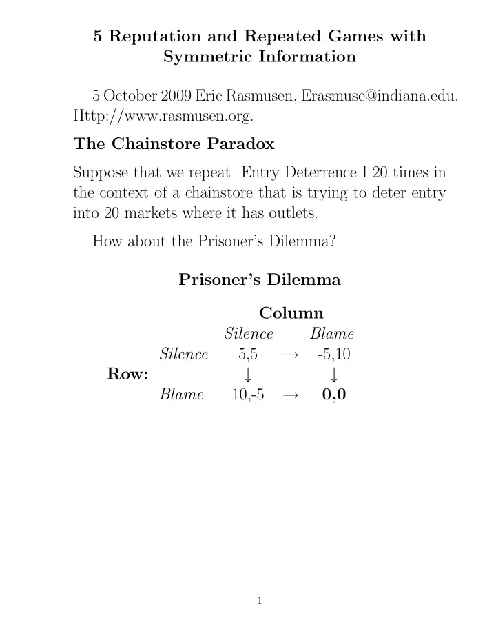
5 Reputation and Repeated Games with Symmetric Information 5 October 2009 Eric Rasmusen, Erasmuse@indiana.edu. Http://www.rasmusen.org. The Chainstore Paradox Suppose that we repeat Entry Deterrence I 20 times in the context of a chainstore that is trying to deter entry into 20 markets where it has outlets. How about the Prisoner’s Dilemma? Prisoner’s Dilemma Column Silence Blame Silence 5,5 →

• 5,10

Row: ↓ ↓ Blame 10,-5 → 0,0

1

Because the one-shot Prisoner’s Dilemma has a dominant- strategy equilibrium, blaming is the only Nash outcome for the repeated Prisoner’s Dilemma, not just the only perfect outcome. The backwards induction argument does not prove that blaming is the unique Nash outcome. Here is why blaming is the only Nash outcome:

• 1. No strategy in the class that calls for Silence in

the last period can be a Nash strategy, because the same strategy with Blame replacing Silence would dominate it.

• 2. If both players have strategies calling for blaming

in the last period, then no strategy that does not call for blaming in the next-to-last period is Nash, because a player should deviate by replacing Silence with Blame in the next- to-last period. Uniqueness is only on the equilibrium path. Nonper- fect Nash strategies could call for cooperation at nodes away from the equilibrium path. The strategy of always blaming is not a dominant strategy. If the one-shot game has multiple Nash equilibria, the perfect equilibrium of the finitely repeated game can have not only the one-shot outcomes, but others besides. See Benoit & Krishna (1985).

2

What if we repeat the Prisoner’s Dilemma an infinite number of times? Defining payoffs in games that last an infinite number

• f periods presents the problem that the total payoff is

infinite for any positive payment per period. 1 Use an overtaking criterion. Payoff stream π is preferred to ˜ π if there is some time T ∗ such that for every T ≥ T ∗,

T

• t=1

δtπt >

T

• t=1

δt ˜ πt. 2 Specify that the discount rate is strictly positive, and use the present value. Since payments in distant periods count for less, the discounted value is finite unless the payments are growing faster than the discount rate. 3 Use the average payment per period, a tricky method since some sort of limit needs to be taken as the number

• f periods averaged goes to infinity.

3

Here is a strategy that yields an equilibrium with SI- LENCE. The Grim Strategy 1 Start by choosing Silence. 2 Continue to choose Silence unless some player has chosen Blame, in which case choose Blame forever. THe GRIM STRATEGY is an example of a trigger strategy. Porter (1983b), who examines price wars between rail- roads in the 19th century. Slade (1987) concluded that price wars among gas stations in Vancouver used small punishments for small deviations rather than big punishments for big devia- tions.

4

Not every strategy that punishes blaming is perfect. A notable example is the strategy of Tit-for-Tat. Tit-for-Tat 1 Start by choosing Silence. 2 Thereafter, in period n choose the action that the

• ther player chose in period (n − 1).

Tit-for-Tat is almost never perfect in the infinitely repeated Prisoner’s Dilemma because it is not rational for Column to punish Row’s initial Blame. The deviation that kills the potential equilibrium is not from Silence, but from the off-equilibrium action rule of Blame in response to a Blame. Adhering to Tit-for-Tat’s punishments results in a miserable alternation of Blame and Silence, so Col- umn would rather ignore Row’s first Blame. Problem 5.5 asks you to show this formally.

5

Theorem 1 (the Folk Theorem) In an infinitely repeated n-person game with finite action sets at each repetition, any profile of actions

• bserved in any finite number of repetitions is the

unique outcome of some subgame perfect equilibrium given Condition 1: The rate of time preference is zero,

• r positive and sufficiently small;

Condition 2: The probability that the game ends at any repetition is zero, or positive and sufficiently small; and Condition 3: The set of payoff profiles that strictly Pareto dominate the minimax payoff profiles in the mixed extension of the one-shot game is n- dimen- sional.

6

Condition 1: Discounting The Grim Strategy imposes the heaviest possible pun- ishment for deviant behavior. : Prisoner’s Dilemma Column Silence Blame Silence 5,5 →

• 5,10

Row: ↓ ↓ Blame 10,-5 → 0,0 π(equilibrium) = 5 + 5 r π(BLAME) = 10 + 0 These are equal at r = 1 , so δ =

1 1+r = .5

7

Condition 2: A probability of the game ending If θ > 0, the game ends in finite time with probability

• ne; or, put less dramatically, the expected number of

repetitions is finite. Ending in finite time with probability one means that the limit of the probability the game has ended by date t approaches one as t tends to infinity; the probability that the game lasts till infinity is zero. Equivalently, the expectation of the end date is finite, which it could not be were there a positive probability

• f an infinite length.

It still behaves like a discounted infinite game, be- cause the expected number of future repetitions is always large, no matter how many have already occurred. It is “stationary”. The game still has no Last Period, and it is still true that imposing one, no matter how far beyond the ex- pected number of repetitions, would radically change the results. “1 The game will end at some uncertain date before T.” “2 There is a constant probability of the game ending.”

8

From Amazing Grace: When we’ve been there ten thousand years, Bright shining as the sun, We’ve no less days to sing God’s praise Than when we’d first begun.

9

Condition 3: Dimensionality The “minimax payoff” is the payoff that results if all the

• ther players pick strategies solely to punish player i,

and he protects himself as best he can. The set of strategies si∗

−i is a set of (n−1) minimax

strategies chosen by all the players except i to keep i’s payoff as low as possible, no matter how he responds. si∗

−i solves Minimize

s−i

Maximum

si πi(si, s−i). (1) Player i’s minimax payoff, minimax value, or security value: his payoff from this.

10

The dimensionality condition is needed only for games with three or more players. It is satisfied if there is some payoff profile for each player in which his payoff is greater than his minimax payoff but still different from the payoff of every other player. Thus, a 3-person Ranked Coordination game would fail it. The condition is necessary because establishing the desired behavior requires some way for the other players to punish a deviator without punishing themselves. Figure 1: The Dimensionality Condition

11

Minimax and Maximin The strategy s∗

i is a maximin strategy for player

i if, given that the other players pick strategies to make i’s payoff as low as possible, s∗

i gives i the high-

est possible payoff. In our notation, s∗

i solves Maximize

si

Minimum

s−i πi(si, s−i). (2) The minimax and maximin strategies for a two-player game with Player 1 as i: Maximin: Maximum Minimum π1 s1 s2 Minimax: Minimum Maximum π1 s2 s1 In the Prisoner’s Dilemma, the minimax and max- imin strategies are both Blame.

12

The minimax and maximin strategies for a two-player game with Player 1 as i: Maximin: Maximum Minimum π1 s1 s2 Minimax: Minimum Maximum π1 s2 s1 Under minimax, Player 2 is purely malicious but must move first (at least in choosing a mixing probability) in his attempt to cause player 1 the maximum pain. Under maximin, Player 1 moves first, in the belief that Player 2 is out to get him. In variable-sum games, minimax is for sadists and maximin for paranoids. In zero-sum games, the players are merely neurotic. Minimax is for optimists, and maximin is for pessimists. The maximin strategy need not be unique, and it can be in mixed strategies. Since maximin behavior can also be viewed as min- imizing the maximum loss that might be suffered, de- cision theorists refer to such a policy as a minimax criterion.

13

Minimax and maximin strategies are not always pure strategies. In the Minimax Illustration Game Row can guarantee himself a payoff of 0 by choosing Down, so that is his maximin strategy. Column cannot hold Row’s payoff down to 0 by using a pure minimax strategy. If Column chooses Left, Row can choose Middle and get a payoff of 1; if Column chooses Right, Row can choose Up and get a payoff of 1. Column can, however, hold Row’s payoff down to 0 by choosing a mixed minimax strategy of (Probability 0.5 of Left, Probability 0.5 of Right). Row would then respond with Down, for a minimax payoff of 0, since either Up, Middle, or a mixture of the two would give him a payoff of −0.5 (= 0.5(−2)+0.5(1)). Table 1: The Minimax Illustration Game Column Left Right Up −2, 2 1 , −2 Row: Middle 1 , −2 −2, 2 Down 0, 1 0, 1

14

The Minimax Illustration Game Column Left Right Up −2, 2 1 , −2 Row: Middle 1 , −2 −2, 2 Down 0, 1 0, 1 Row’s strategy for minimaxing Column is (Probabil- ity 0.5 of Up, Probability 0.5 of Middle). Row’s maximin strategy is (Probability 0.5 of Left, Probability 0.5 of Right), and his minimax payoff is 0. The Minimax Theorem (von Neumann [1928]), says that a minimax equilibrium exists in pure or mixed strategies for every two-person zero-sum game and is identical to the maximin equilibrium.

15

Precommitment What if we allow players to commit at the start to a strategy for the rest of the game? If precommitted strategies are chosen simultaneously, the equilibrium outcome of the finitely repeated Pris-

• ner’s Dilemma calls for always blaming.

What about in sequence? The outcome depends on the particular values of the parameters, but one possible equilibrium is the following: Row moves first and chooses the strategy (Silence un- til Column Blames; thereafter always Blame), and Col- umn chooses (Silence until the last period; then Blame). The observed outcome would be for both players to choose Silence until the last period, and then for Row to again choose Silence , but for Column to choose Blame . Row would submit to this because if he chose a strategy that initiated blaming earlier, Column would choose a strategy of starting to blame earlier too. The game has a second-mover advantage.

16

The One-Sided Prisoner’s Dilemma (Reputation) Consumer (Column) Buy Boycott High Quality 5,5 ← 0,0 Seller (Row): ↓

• Low Quality

10, -5 → 0,0 The Nash and iterated dominance equilibria are (Blame, Blame), but it is not a dominant-strategy equilibrium. Column does not have a dominant strategy, because if Row were to choose Silence, Column would also choose Silence, to obtain the payoff of 5; but if Row chooses Blame, Column would choose Blame, for a payoff of zero. Blame is however, weakly dominant for Row, which makes (Blame, Blame) the iterated dominant strategy equilibrium.

17

Product Quality, Klein & Leffler (1981) The Order of Play 1 An endogenous number n of firms decide to enter the market at cost F. 2 A firm that has entered chooses its quality to be High

• r Low, incurring the constant marginal cost c if it picks

High and zero if it picks Low. The choice is unobserved by consumers. The firm also picks a price p. 3 Consumers decide which firms (if any) to buy from, choosing firms randomly if they are indifferent. The amount bought from firm i is denoted qi. 4 All consumers observe the quality of all goods pur- chased in that period. 5 The game returns to (2) and repeats. Payoffs The consumer benefit from a product of low quality is zero, but consumers are willing to buy quantity q(p) = n

i=1 qi for a product believed to be high quality, where dq dp < 0.

If a firm stays out of the market, its payoff is zero. If firm i enters, it receives −F immediately. Its current end-of- period payoff is qip if it produces Low quality and qi(p − c) if it produces High quality. The discount rate is r ≥ 0.

18

An equilibrium:

• Firms. ˜

n firms enter. Each produces high quality and sells at price ˜ p. If a firm ever deviates from this, it thereafter produces low quality (and sells at the same price ˜ p). Buyers. Buyers start by choosing randomly among the firms charging ˜

• p. Thereafter, they remain with their

initial firm unless it changes its price or quality, in which case they switch randomly to a firm that has not changed its price or quality.

19

For this story to work, however, the equilibrium must satisfy three constraints that will be explained in more depth in Section 7.3: incentive compatibility, competi- tion, and market clearing. The incentive compatibility constraint says that the individual firm must be willing to produce high qual- ity. qip 1 + r ≤ qi(p − c) r (incentive compatibility). (3) Firms must be willing to ˜ p ≥ (1 + r)c. (4) The second constraint is that competition drives prof- its to zero, so firms are indifferent between entering and staying out of the market. qi(p − c) r = F (competition) (5) Treating (3) as an equation and using it to replace p in equation (5) gives qi = F c . (6) Third, the output must equal the quantity demanded by the market. nqi = q(p). (market clearing) (7)

20

Combining equations (3), (6), and (7) yields ˜ n = cq([1 + r]c) F . (8) What if there were no entry cost? Would profits be dissipated?

21

Reputation: Umbrella Branding I’ll present my paper with Myatt.

22

Customer Switching Costs, Farrell & Shapiro (1988) Players Firms Apex and Brydox, and a series of customers, each

• f whom is first called a youngster and then an oldster.

The Order of Play 1a Brydox, the initial incumbent, picks the incumbent price pi

1.

1b Apex, the initial entrant, picks the entrant price pe

1.

1c The oldster picks a firm. 1d The youngster picks a firm. 1e Whichever firm attracted the youngster becomes the incumbent. 1f The oldster dies and the youngster becomes an old- ster. 2a Return to (1a), possibly with new identities for en- trant and incumbent. Payoffs The discount factor is δ. The customer reservation price is R and the switching cost is c. The per period payoffs in period t are, for j = (i, e), πfirm j =    if no customers are attracted. pj

t

if just oldsters or just youngsters are attra 2pj

t if both oldsters and youngsters are attracted.

23

πoldster = R − pi

t

if he buys from the incumbent. R − pe

t − c if he switches to the entrant.

πyoungster = R − pi

t if he buys from the incumbent.

R − pe

t if he buys from the entrant.

24

A Markov strategy is a strategy that, at each node, chooses the action independently of the history

• f the game except for the immediately preceding ac-

tion (or actions, if they were simultaneous). Here, a firm’s Markov strategy is its price as a function

• f whether the particular is the incumbent or the entrant,

and not a function of the entire past history of the game. There are two ways to use Markov strategies: (1) just look for equilibria that use Markov strategies (perfect Markov equilibrium ) (2) disallow non-Markov strategies and then look for equilibria.

25

Brydox, the initial incumbent, moves first and chooses pi low enough that Apex is not tempted to choose pe < pi−c and steal away the oldsters. Apex’s profit is pi if it chooses pe = pi and serves just youngsters, and 2(pi −c) if it chooses pe = pi − c and serves both oldsters and

• youngsters. Brydox chooses pi to make Apex indifferent

between these alternatives, so pi = 2(pi − c), (9) and pi = pe = 2c. (10) In equilibrium, Apex and Brydox take turns being the incumbent and charge the same price. The equilibrium payoff of the current entrant is the immediate payment of pe plus the discounted value of being the incumbent in the next period: π∗

e = pe + δπ∗ i .

(11) The incumbent’s payoff can be similarly stated as the immediate payment of pi plus the discounted value of being the entrant next period: π∗

i = pi + δπ∗ e.

(12) In equilibrium the incumbent and the entrant sell the same amount at the same price, so π∗

i = π∗ e and

π∗

i = 2c + δπ∗ i .

(13)

26

It follows that π∗

i = π∗ e =

2c 1 − δ. (14)

27

*5.6 Evolutionary Equilibrium: Hawk-Dove A strategy s∗ is an evolutionarily stable strategy,

• r ESS, if, using the notation π(si, s−i) for player i’s

payoff when his opponent uses strategy s−i, for every

• ther strategy s′ either

π(s∗, s∗) > π(s′, s∗) (15)

• r

(a) π(s∗, s∗) = π(s′, s∗) and (b) π(s∗, s′) > π(s′, s′). (16) If condition (17) holds, then a population of players using s∗ cannot be invaded by a deviant using s′. If condition (18) holds, then s′ does well against s∗, but badly against itself, so that if more than one player tried to use s′ to invade a population using s∗, the invaders would fail.

28

A strategy s∗ is an evolutionarily stable strategy,

• r ESS, if, using the notation π(si, s−i) for player i’s

payoff when his opponent uses strategy s−i, for every

• ther strategy s′ either

π(s∗, s∗) > π(s′, s∗) (17)

• r

(a) π(s∗, s∗) = π(s′, s∗) and (b) π(s∗, s′) > π(s′, s′). (18) Condition (17) says that s∗ is a strong Nash equi- librium (although not every strong Nash strategy is an ESS). Condition (18) says that if s∗ is only a weak Nash strategy, the weak alternative s′ is not a best response to itself. ESS is a refinement of Nash: Nash plus: (a) it has the highest payoff of any strategy used in equilibrium (which rules out equilibria with asymmetric payoffs), (b) it is a strictly best response to itself

29

ESS is a refinement of Nash: Nash plus: (a) it has the highest payoff of any strategy used in equilibrium (which rules out equilibria with asymmetric payoffs), (b) it is a strictly best response to itself (a) CThe Battle of the Sexes. In it, the mixed strategy equilibrium is an ESS, because a player using it has as high a payoff as any other player. The two pure strategy equilibria are not made up of ESS’s, though, because in each of them one player’s payoff is higher than the

• ther’s. Compare with Ranked Coordination, in which

the two pure strategy equilibria and the mixed strat- egy equilibrium are all made up of ESS’s. (The dom- inated equilibrium strategy is nonetheless an ESS, be- cause given that the other players are using it, no player could do as well by deviating.)

30

(b) The Utopian Exchange Economy. In Utopia, each citizen can produce either one or two units of individu- alized output. He will then go into the marketplace and meet another citizen. If either of them produced only

• ne unit, trade cannot increase their payoffs. If both of

them produced two, however, they can trade one unit for

• ne unit, and both end up happier with their increased

variety of consumption. Table 4 The Utopian Exchange Economy Game Jones Low Output HighOutput LowOutput 1, 1 ↔ 1, 1 Smith:

• ↓

High Output 1,1 → 2,2 This game has three Nash equilibria, one of which is in mixed strategies. Since all strategies but High Output are weakly dominated, that alone is an ESS. Low Output fails to meet condition (b), because it is not the strictly best response to itself. If the economy began with all citizens choosing Low Output, then if Smith deviated to High Output he would not do any better, but if two people deviated to High Output, they would do better in expectation because they might meet each other and receive the payoff of

31

(2,2).

32

An Example of ESS: Hawk-Dove A resource worth V = 2 “fitness units” is at stake when the two birds meet. If they both fight, the loser incurs a cost of C = 4, which means that the expected payoff when two Hawks meet is −1 (= 0.5[2] + 0.5[−4]) for each of them. . Table 5 Hawk-Dove: Economics Notation Bird Two Hawk Dove Hawk

• 1,-1

→ 2,0 Bird One: ↓ ↑ Dove 0, 2 ← 1,1 Payoffs to: (Bird One, Bird Two). Arrows show how a player can increase his payoff. Table 6 Hawk-Dove: Biology Notation Bird Two Hawk Dove Hawk

• 1

2 Bird One: Dove 1 Payoffs to: (Bird One)

33

Hawk-Dove has no symmetric pure-strategy Nash equi- librium, and hence no pure-strategy ESS, since in the two asymmetric Nash equilibria, Hawk gives a bigger pay-

• ff than Dove, and the doves would disappear from the

population. In the mixed-strategy ESS, the equilibrium strategy is to be a hawk with probability 0.5 and a dove with probability 0.5, which can be interpreted as a population 50 percent hawks and 50 percent doves. The equilibrium is stable in a sense similar to the Cournot equilibrium. If 60 percent of the population were hawks, a bird would have a higher fitness level as a

• dove. If “higher fitness” means being able to reproduce

faster, the number of doves increases and the proportion returns to 50 percent over time.

34

The bourgeois strategy (a correlated strategy) is an ESS. Under this strategy, the bird behaves as a hawk if it arrives first, and a dove if it arrives second. The bourgeois strategy has an expected payoff of 1 from meeting itself, and behaves exactly like a 50:50 ran- domizer when it meets a strategy that ignores the order

• f arrival, so it can successfully invade a population of

50:50 randomizers.

35

The ESS is suited to games in which all the players are identical and interacting in pairs. The approach follows three steps: (1) the initial population proportions and the probabili- ties of interactions, (2) the pairwise interactions, (3) the dynamics by which players with higher payoffs increase in number in the population.

36

Slow dynamics also makes the starting point of the game important, unlike the case when adjustment is instantaneous. Figure 2, taken from David Friedman (1991), shows a way to graphically depict evolution in a game in which all three strategies of Hawk, Dove, and Bourgeois are used. A point in the triangle represents a proportion of the three strategies in the population. At point E3, for example, half the birds play Hawk, half play Dove, and none play Bourgeois, while at E4 all the birds play Bourgeois. Evolutionary Dynamics in the Hawk-Dove-

37

Bourgeois Game Figure 2 also shows the importance of mutation in bi-

• logical games. If the population of birds is 100 percent

dove, as at E2, it stays that way in the absence of muta- tion, since if there are no hawks to begin with, the fact that they would reproduce at a faster rate than doves becomes irrelevant.

38