3D Deep Learning on Geometric Forms Hao Su Many 3D representations - PowerPoint PPT Presentation

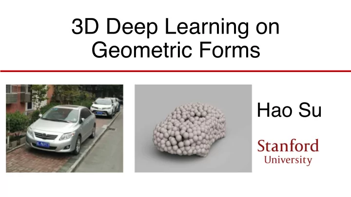
3D Deep Learning on Geometric Forms Hao Su

Many 3D representations are available Candidates: multi-view images depth map volumetric polygonal mesh point cloud primitive-based CAD models

3D representation Candidates: multi-view images depth map volumetric polygonal mesh point cloud primitive-based CAD models Novel view image synthesis [Su et al., ICCV15] [Dosovitskiy et al., ECCV16]

3D representation Candidates: multi-view images depth map volumetric polygonal mesh point cloud primitive-based CAD models

3D representation Candidates: multi-view images depth map volumetric polygonal mesh point cloud primitive-based CAD models

3D representation Candidates: multi-view images depth map volumetric polygonal mesh point cloud primitive-based CAD models

3D representation Candidates: multi-view images depth map volumetric polygonal mesh point cloud primitive-based CAD models

3D representation Candidates: multi-view images depth map volumetric polygonal mesh point cloud primitive-based CAD models a chair assembled by cuboids

Two groups of representations Candidates: multi-view images Rasterized form depth map (regular grids) volumetric polygonal mesh Geometric form point cloud (irregular) primitive-based CAD models

Extant 3D DNNs work on grid-like representations Candidates: multi-view images depth map volumetric polygonal mesh point cloud primitive-based CAD models

Ideally, a 3D representation should be Friendly to learning • easily formulated as the input/output of a neural network • fast forward-/backward- propagation • etc.

Ideally, a 3D representation should be Friendly to learning • easily formulated as the input/output of a neural network • fast forward-/backward- propagation • etc. Flexible • can precisely model a great variety of shapes • etc.

Ideally, a 3D representation should be Friendly to learning • easily formulated as the output of a neural network • fast forward-/backward- propagation • etc. Flexible • can precisely model a great variety of shapes • etc. Geometrically manipulable for networks • geometrically deformable, interpolable and extrapolable for networks • convenient to impose structural constraints • etc. Others

The problem of grid representations Affability Geometric Flexibility to learning manipulability Multi-view images Volumetric occupancy Expensive to compute: O(N 3 ) Depth map Cannot model “back side”

Typical artifacts of volumetric reconstruction Missing or extra thin structures Volumes are hard for the network to rotate / deform / interpolate

Learn to analyze / generate Geometric Forms? Candidates: multi-view images Rasterized form depth map (regular grids) volumetric polygonal mesh Geometric form point cloud (irregular) primitive-based CAD models

Outline Motivation 3D point cloud / CAD model reconstruction 3D point cloud analysis, e.g., segmentation

3D point clouds A dual formulation of occupancy Flexibility Geometric manipulability Affability to learning Lagrangian Eulerian Prob. distribution Particle filters Volumetric Point occupancy clouds

Result: 3D reconstruction from real Images Input Reconstructed 3D point cloud

Result: 3D reconstruction from real Images Input Reconstructed 3D point cloud

An end-to-end synthesis-for-learning system Image rendering   ( x 0 1 , y 0 1 , z 0 1 )     ( x 0 2 , y 0 2 , z 0 2 )   ... sampling     ( x 0 n , y 0 n , z 0 n )   3D model Groundtruth point cloud

An end-to-end learning system Image Predicted set   ( x 1 , y 1 , z 1 )     Deep Neural ( x 2 , y 2 , z 2 )   Network ...     ( x n , y n , z n )     ( x 0 1 , y 0 1 , z 0 1 )     ( x 0 2 , y 0 2 , z 0 2 )   ...     ( x 0 n , y 0 n , z 0 n )   Groundtruth point cloud

An end-to-end learning system Image Predicted set   ( x 1 , y 1 , z 1 )     Deep Neural ( x 2 , y 2 , z 2 )   Network ...     ( x n , y n , z n )   Point Set Distance   ( x 0 1 , y 0 1 , z 0 1 )     ( x 0 2 , y 0 2 , z 0 2 )   ...     ( x 0 n , y 0 n , z 0 n )   Groundtruth point cloud

An end-to-end learning system Image Predicted set   ( x 1 , y 1 , z 1 )     Deep Neural ( x 2 , y 2 , z 2 )   Network ...     ( x n , y n , z n )   Point Set Distance   ( x 0 1 , y 0 1 , z 0 1 )     ( x 0 2 , y 0 2 , z 0 2 )   ...     ( x 0 n , y 0 n , z 0 n )   Groundtruth point cloud

Network architecture: Vanilla version Fully connected layer as predictor in standard classification network fully connected conv Encoder input shape embedding ! " point set Predictor

Network architecture: Vanilla version Fully connected layer as predictor in standard classification network fully connected conv Encoder input shape embedding ! " point set Predictor & ! " Independently regress n*3 numbers from : #×3

Natural statistics of geometry • Many objects, especially man-made objects, contain large smooth surfaces • Deconvolution can generate locally smooth textures for images

Network architecture: Output from deconv branch Two branch version conv deconv fully connected set union input Encoder # ' =24*32=768 points Predictor point set # ( =256 points 3-channel map of XYZ coordinates

Network architecture: Output from deconv branch Two branch version conv deconv fully connected set union input Encoder # ' =24*32=768 points Predictor point set # ( =256 points 3-channel map of XYZ coordinates  C 1 C 1 ∈ R n 1 × 3 � C = C 2 ∈ R n 2 × 3 C 2

Network architecture: Output from deconv branch Two branch version conv deconv fully connected set union input Encoder # ' =24*32=768 points Predictor point set # ( =256 points 3-channel map of XYZ coordinates

Network architecture: The role of two branches blue : deconv branch – large, consistent, smooth structures red : fully-connected branch – flexibly reconstruct intricate structures

An end-to-end learning system Predicted set   ( x 1 , y 1 , z 1 )     Deep Neural ( x 2 , y 2 , z 2 )   Network ...     ( x n , y n , z n )   Point Set Loss   ( x 0 1 , y 0 1 , z 0 1 )     ( x 0 2 , y 0 2 , z 0 2 )   ...     ( x 0 n , y 0 n , z 0 n )   Groundtruth point cloud

Distance metrics between point sets Given two sets of points, measure their discrepancy

Common distance metrics Worst case: Hausdorff distance (HD) Average case: Chamfer distance (CD) Optimal case: Earth Mover’s distance (EMD)

Common distance metrics Worst case: Hausdorff distance (HD) d HD( S 1 , S 2 ) = max { max x i ∈ S 1 min y j ∈ S 2 k x i � y j k , max y j ∈ S 2 min x i ∈ S 1 k x i � y j k } A single farthest pair determines the distance. In other words, not robust to outliers!

Common distance metrics Worst case: Hausdorff distance (HD) Average case: Chamfer distance (CD) Average all the nearest neighbor distance by nearest neighbors

Common distance metrics Worst case: Hausdorff distance (HD) Average case: Chamfer distance (CD) Optimal case: Earth Mover’s distance (EMD) Solves the optimal transportation (bipartite matching) problem!

Required properties of distance metrics Geometric requirement • Induces a nice shape space • In other words, a good metric should reflect the natural shape differences Computational requirement • Defines a loss that is numerically easy to optimize

Required properties of distance metrics Geometric requirement • Induces a nice shape space • In other words, a good metric should reflect the natural shape differences Computational requirement • Defines a loss that is numerically easy to optimize

How distance metric affects the learned geometry? A fundamental issue: there is always uncertainty in prediction By loss minimization, the network tends to predict a “ mean shape ” that averages out uncertainty in geometry

How distance metric affects the learned geometry? A fundamental issue: there is always uncertainty in prediction, due to • limited network ability • Insufficient training data • inherent ambiguity of groundtruth for 2D-3D dimension lifting • etc. By loss minimization, the network tends to predict a “ mean shape ” that averages out uncertainty in geometry

Mean shapes are affected by distance metric The mean shape carries characteristics of the distance metric x = argmin ¯ E s ∼ S [ d ( x, s )] x continuous hidden variable (radius) Input EMD mean Chamfer mean

Mean shapes from distance metrics The mean shape carries characteristics of the distance metric x = argmin ¯ E s ∼ S [ d ( x, s )] x continuous hidden variable (radius) discrete hidden variable (add-on location) Input EMD mean Chamfer mean

Comparison of predictions by CD versus EMD Chamfer EMD Input