3264 CONICS IN A SECOND Paul Breiding Bernd Sturmfels Sascha - PowerPoint PPT Presentation

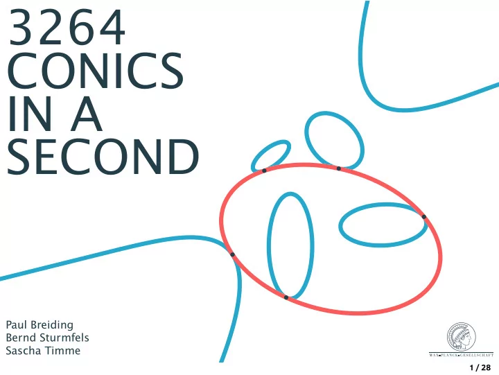
3264 CONICS IN A SECOND Paul Breiding Bernd Sturmfels Sascha Timme 1 / 28

A conic in the plane R 2 is the set of solutions to a quadratic equation A ( x, y ) = 0 , where A ( x, y ) = a 1 x 2 + a 2 xy + a 3 y 2 + a 4 x + a 5 y + 1 . 2 / 28

A second conic U ( x, y ) = u 1 x 2 + u 2 xy + u 3 y 2 + u 4 x + u 5 y + 1 , is tangent to A if there exists ( x, y ) such that   ∂A ∂U ∂x ∂x  = 0 . A ( x, y ) = 0 , U ( x, y ) = 0 det and  ∂A ∂U ∂y ∂y 3 / 28

Eliminating ( x, y ) from  ∂A ∂U  ∂x ∂x  = 0 A ( x, y ) = 0 , U ( x, y ) = 0 det and  ∂A ∂U ∂y ∂y we get the tact invariant : T ( A, U ) = 256 a 4 1 a 2 3 u 2 3 − 128 a 4 1 a 2 3 u 3 u 2 5 + 16 a 4 1 a 2 3 u 4 5 − 256 a 4 1 a 3 a 5 u 2 3 u 5 + 128 a 4 1 a 3 a 5 u 3 u 3 5 − 16 a 4 1 a 3 a 5 u 5 5 − 512 a 4 1 a 3 1 u 3 3 + · · · + a 4 5 u 2 1 u 4 2 . For fixed u 1 . . . , u 5 the tact invariant T ( A, U ) is a polynomial of degree 6 in the 5 variables a 1 , . . . , a 5 . 4 / 28

Counting degrees of freedom we see that there are finitely many conics tangent to 5 fixed conics. 5 / 28

How many conics? The question How many? started the modern development of enumerative geometry. Recall: T ( A, U ) is a polynomial of degree 6 in 5 variables . Based on this, Jakob Steiner claimed in 1848 that there are 6 5 = 7776 (complex) conics tangent to five conics. In 1864 Michel Chasles gave the correct answer of 3264 . 6 / 28

Why was Steiner wrong? He missed that there is a Veronese surface of extraneous solutions, namely the conics that are squares of linear forms . 7 / 28

Why was Steiner wrong? He missed that there is a Veronese surface of extraneous solutions, namely the conics that are squares of linear forms . How do we fix this? 7 / 28

Why was Steiner wrong? He missed that there is a Veronese surface of extraneous solutions, namely the conics that are squares of linear forms . How do we fix this? We replace P 5 C with another five-dimensional manifold, namely the compact space of complete conics . This is the blow-up of P 5 C at the locus of double conics. 7 / 28

Why was Steiner wrong? He missed that there is a Veronese surface of extraneous solutions, namely the conics that are squares of linear forms . How do we fix this? We replace P 5 C with another five-dimensional manifold, namely the compact space of complete conics . This is the blow-up of P 5 C at the locus of double conics. To answer enumerative geometry questions we work in the Chow ring of the space of complete conics. 7 / 28

Applying intersection theory This Chow ring contains three special classes P and L : 1 P encodes the conics passing through a fixed point 2 L encodes the conics tangent to a fixed line 3 C encodes the conics tangent to a given conic 8 / 28

Applying intersection theory This Chow ring contains three special classes P and L : 1 P encodes the conics passing through a fixed point 2 L encodes the conics tangent to a fixed line 3 C encodes the conics tangent to a given conic The following relations hold: P 5 = L 5 = 1 , P 4 L = PL 4 = 2 and P 3 L 2 = P 2 L 3 = 4 . C = 2 P + 2 L (this requires a proof) 8 / 28

Applying intersection theory This Chow ring contains three special classes P and L : 1 P encodes the conics passing through a fixed point 2 L encodes the conics tangent to a fixed line 3 C encodes the conics tangent to a given conic The following relations hold: P 5 = L 5 = 1 , P 4 L = PL 4 = 2 and P 3 L 2 = P 2 L 3 = 4 . C = 2 P + 2 L (this requires a proof) The desired intersection number is now obtained from the Binomial Theorem: C 5 = 2 5 · ( L + P ) 5 = 2 5 · ( L 5 + 5 L 4 P + 10 L 3 P 2 + 10 L 2 P 3 + 5 LP 4 + P 5 ) = 2 5 · (1 + 5 · 2 + 10 · 4 + 10 · 4 + 5 · 2 + 1) = 32 · 102 = 3264 . 8 / 28

What about real solutions? This yields the question: Is there an instance of Steiner’s problem whose 3264 solutions are all real ? 9 / 28

What about real solutions? This yields the question: Is there an instance of Steiner’s problem whose 3264 solutions are all real ? The answer is YES! This was first observed by Fulton, and worked out in detail by Ronga, Tognoli and Vust, and Sottile. 9 / 28

Constructing 3264 real solutions We start with 5 double lines, forming a pentagon. 10 / 28

Constructing 3264 real solutions We start with 5 double lines, forming a pentagon. 10 / 28

Constructing 3264 real solutions Mark a special point on each edge. 10 / 28

Constructing 3264 real solutions There are 102 = ( L + P ) 5 conics which are tangent to a subset of the lines and going through the other special points. 10 / 28

Constructing 3264 real solutions There are 102 = ( L + P ) 5 conics which are tangent to a subset of the lines and going through the other special points. 10 / 28

Constructing 3264 real solutions By a small perturbation each of the 102 conic splits into 32 solutions. 11 / 28

Constructing 3264 real solutions By a small perturbation each of the 102 conic splits into 32 solutions. But what is small ? 11 / 28

Constructing 3264 real solutions By a small perturbation each of the 102 conic splits into 32 solutions. But what is small ? Can we find a concrete instance and give a proof that it has 3264 real solutions? 11 / 28

Numerical Algebraic Geometry 12 / 28

Homotopy Continuation Homotopy continuation is a technique for 5 numerically solving systems of polynomial equations. Essentially, for solving a system F = ( f 1 ( x 1 , . . . , x n ) , . . . , f n ( x 1 , . . . , x n )) it does the following: take another system G = ( g 1 ( x 1 , . . . , x n ) , . . . , g n ( x 1 , . . . , x n )) , of which we know all zeros. Then track the zeros along a path H ( x, t ) H ( x, 1) = G ( x ) , H ( x, 0) = F ( x ) with towards F . 13 / 28

Homotopy Continuation Cartoon X -axis = space of polynomial systems. Y -axis = space of zeros. 14 / 28

Path Tracking We have to track the zeros x ( t ) from t = 1 towards t = 0 . From H ( x ( t ) , t ) = 0 for t ∈ [0 , 1] follows that x ( t ) can be described by the Davidenko differential equation H x ( x ( t ) , t ) ˙ x ( t ) + H t ( x ( t ) , t ) = 0 Given a solution x 1 = x (1) this is an initial value problem . 15 / 28

Predictor Corrector Scheme Given some discretization 1 = t 0 > t 1 > . . . > t K = 0 we can follow a path numerically using a predictor- corrector scheme . 16 / 28

Predictor Corrector Scheme Given some discretization 1 = t 0 > t 1 > . . . > t K = 0 we can follow a path numerically using a predictor- corrector scheme . ~ x k +1 corrector predictor ~ x k +2 x(t) t t k t k +2 k +1 The corrector is usually Newton’s method. 16 / 28

Computing all zeros We can compute all zeros of a polynomial system F by embedding it in a larger family of polynomial systems where we can compute all solutions. Examples : • Bezout’s theorem (total degree homotopy) • Bernstein-Kushnirenko theorem (polyhedral homotopy) 17 / 28

Computing all zeros We can compute all zeros of a polynomial system F by embedding it in a larger family of polynomial systems where we can compute all solutions. Examples : • Bezout’s theorem (total degree homotopy) • Bernstein-Kushnirenko theorem (polyhedral homotopy) Another method for polynomial systems with parametric coefficients is based on the monodromy action induced by the fundamental group of the regular locus of the parameter space. 17 / 28

Monodromy - Theory Assume F p is a polynomial system in n variables with parametric coefficients depending on p = ( p 1 , . . . , p m ) . 18 / 28

Monodromy - Theory Assume F p is a polynomial system in n variables with parametric coefficients depending on p = ( p 1 , . . . , p m ) . Consider the variety Y := { ( x, p ) ∈ C n × C m | F p ( x ) = 0 } and assume there exists an open set Q ⊂ C m such that π : Y → Q, ( x, p ) → p has generically finite fibers of degree D . 18 / 28

Monodromy - Theory Assume F p is a polynomial system in n variables with parametric coefficients depending on p = ( p 1 , . . . , p m ) . Consider the variety Y := { ( x, p ) ∈ C n × C m | F p ( x ) = 0 } and assume there exists an open set Q ⊂ C m such that π : Y → Q, ( x, p ) → p has generically finite fibers of degree D . A loop in Q based at q has D lifts to π − 1 ( Q ) , one for each point in the fiber π − 1 ( q ) . Associating a point in the fiber π − 1 ( q ) to the endpoint of the corresponding lift gives a permutation in S D . 18 / 28

Monodromy - Application If F is a polynomial system with parametric coefficients and we know one solution for a generic parameter q we can use the monodromy action to populate the fiber π − 1 ( q ) . Example : • The conics tangent to five given conics 19 / 28