19 Advanced Topics 1: MT System Combination In the chapters up to - PDF document
19 Advanced Topics 1: MT System Combination In the chapters up to this point, we have covered methods to create e ff ective systems for machine translation. In actuality, when attempting to create the strongest possible system possible, it is
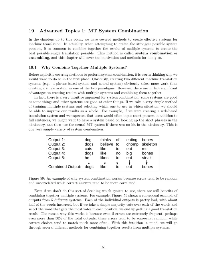
19 Advanced Topics 1: MT System Combination In the chapters up to this point, we have covered methods to create e ff ective systems for machine translation. In actuality, when attempting to create the strongest possible system possible, it is common to combine together the results of multiple systems to create the best possible single translation possible. This method is called system combination or ensembling , and this chapter will cover the motivation and methods for doing so. 19.1 Why Combine Together Multiple Systems? Before explicitly covering methods to perform system combination, it is worth thinking why we would want to do so in the first place. Obviously, creating two di ff erent machine translation systems (e.g. a phrase-based system and neural system) obviously takes more work than creating a single system in one of the two paradigms. However, there are in fact significant advantages to creating results with multiple systems and combining them together. In fact, there is a very intuitive argument for system combination: some systems are good at some things and other systems are good at other things. If we take a very simple method of training multiple systems and selecting which one to use in which situation, we should be able to improve our results as a whole. For example, if we were creating a web-based translation system and we expected that users would often input short phrases in addition to full sentences, we might want to have a system based on looking up the short phrases in the dictionary, and then use the neural MT system if there was no hit in the dictionary. This is one very simple variety of system combination. Output 1: dog thinks of eating bones Output 2: dogs believe to chomp skeleton Output 3: cats like to eat me Output 4: dogs like no big bones Output 5: he likes to eat steak Combined Output: dogs like to eat bones Figure 59: An example of why system combination works: because errors tend to be random and uncorrelated while correct answers tend to be more correlated. Even if we don’t do this sort of deciding which system to use, there are still benefits of combining together multiple systems. For example, Figure 59 shows a conceptual example of outputs from 5 di ff erent systems. Each of the individual outputs is pretty bad, with about half of the words incorrect, but if we take a simple majority vote over each of the words and select the word that gets the most votes in each position, we end up getting a good translation result. The reason why this works is because even if errors are extremely frequent, perhaps even more than 50% of the total outputs, these errors tend to be somewhat random, while correct choices tend to match much more often. With this intuition in mind, we will go through several di ff erent methods for combining together results from multiple systems. 151
19.2 Ensembling Decisions During Decoding One simple but e ff ective way of ensembling systems together that is widely used, particularly in neural machine translation systems, combines together the decisions predicted by multiple systems in the process of predicting the next word to output. Let’s say we have K neural machine translation systems, each of which can calculate a probability distribution of the next word given the input sentence and the previous words P k ( e t | F, e t − 1 ) (190) 1 where P k represents the probability distribution estimated by the k th system. This method takes in these K probability distributions and converts them into a new probability distri- bution P ( e t | F, e t − 1 ), which is finally used when generating translations in the standard 1 fashion. The simplest way that we can combine K probabilities into a single probability is linear interpolation , quite similar to the variety we used when combining together n -gram models with di ff erent orders K 1 X P ( e t | F, e t − 1 K P k ( e t | F, e t − 1 ) = ) . (191) 1 1 k =1 This can also be parameterized so that the interpolation coe ffi cient for each of the models is di ff erent K P ( e t | F, e t − 1 X α k P k ( e t | F, e t − 1 ) = ) (192) 1 1 k =1 under the restriction that all values of α k are between 0 and 1 and add to 1 in order to assure that we have a well-formed probability distribution. It is also possible to perform log-linear interpolation , where we add together the prob- abilities of each model in log space, then perform a softmax to get the final probability: K X P ( e t | F, e t − 1 α k log P k ( e t | F, e t − 1 ) = softmax( )) . (193) 1 1 k =1 Here it is necessary to normalize the probabilities with the softmax after combining them together, as the sum of the log probabilities won’t necessarily result in a well-formed log probability distribution, and thus we need to re-normalize to ensure that the distribution is correct. As a result of this, the values of α k do not necessarily need to add to 1, and can take any values we choose. These methods have a very similar form, but the results are quite di ff erent. Specifically, linear interpolation will tend to favor hypotheses where any one of the models assigns a high score (similar to the logical “or”), while log-linear interpolation will favor hypotheses where all of the models agree (similar to the logical “and”). 57 Thus, when we prefer that all models are able to confirm a solution, we use log-linear interpolation, and when we prefer that models both propose complimentary solutions, we use linear interpolation. 57 Question: Confirm this by noting that happens with each method when calculating the ensembled probability of three events when the probabilities according to model one are { 0 . 6 , 0 . 3 , 0 . 1 } and according to model two are { 0 . 05 , 0 . 3 , 0 . 65 } . 152
19.3 Post-hoc System Combination The method in the previous section is based on combining together multiple models that make decisions about the next word in the sentnece, like neural models. However, let’s say we want to combine together very di ff erent models that make predictions in very di ff erent ways, such as a neural model, a phrase-based model, and a tree-based model. In this case, it is common to first generate hypotheses with each of these di ff erent models, then use these inde- pendently generated hypotheses to select the best possible solution. Within this framework, there are generally two di ff erent ways to combine together hypotheses from di ff erent systems: reranking and generative combination . 19.3.1 Reranking-based Combination Reranking consists of taking the hypotheses generated by each system, and using some mea- sure of their goodness to select the best one. One simple example of reranking would be to generate N hypotheses for each of the K systems, then select the best of these hypotheses according to the overall probability calculated by each of the systems. More formally, we calculate a sample of N hypotheses for each system k : E k = N − max P k ( E | F ) . (194) E Then we decide the overall space of hypotheses that we will consider as the union of all hypotheses generated by each system K [ E = E k . (195) k =1 We define the probability of each hypothesis P ( E | F ) as the linear (Equation 192) or log- linear (Equation 193) interpolation of the model probabilities, and then select the hypothesis that has the highest probability according to these interpolated probabilities ˆ E = argmax P ( E | F ) . (196) E ∈ E 19.3.2 Minimum Bayes Risk One other widely used criterion for choosing hypotheses that is simple yet e ff ective in both single-system and multi-system reranking is the minimum Bayes risk decision criterion [6]. From the minimum risk training in Section 18.3, we can remember that risk is defined as the expected error of a particular hypothesis E P ( ˜ E | F )error( E, ˜ X risk( E, F ) = E ) . (197) ˜ E In contrast to simply taking the hypothesis with the highest posterior probability in Equa- tion 196 (the max a posteriori (MAP) decision rule) minimum Bayes risk decision rule is an alternative that attempts to minimize this risk ˆ E = argmin risk( E, F ) . (198) E ∈ E 153
Recommend
More recommend
Explore More Topics
Stay informed with curated content and fresh updates.
