15 Tree-based MT In this chapter, we will cover methods for - - PDF document

15 Tree-based MT

In this chapter, we will cover methods for sequence-to-sequence mapping that are based on tree structures.

15.1 Motivation for Tree-based Methods

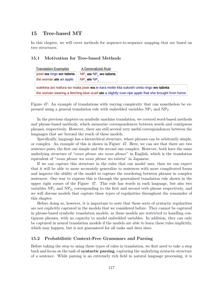
the woman ate an apple josei wa ringo wo tabeta the woman wearing a fetching blue scarf ate a slightly over-ripe apple that she brought from home sutekina aoi mafura wo maita josei wa ie kara motte kita sukoshi ureta ringo wo tabeta NP1 ate NP2 NP1 wa NP2 wo tabeta Translation Examples A Generalized Rule

Figure 47: An example of translations with varying complexity that can nonetheless be ex- pressed using a general translation rule with embedded variables NP1 and NP2. In the previous chapters on symbolic machine translation, we covered word-based methods and phrase-based methods, which memorize correspondences between words and contiguous phrases, respectively. However, there are still several very useful correspondences between the languages that are beyond the reach of these models. Specifically, language has a hierarchical structure, where phrases can be arbitrarily simple,

• r complex. An example of this is shown in Figure 47. Here, we can see that there are two

sentence pairs, the first one simple and the second one complex. However, both have the same underlying structure of “noun phrase ate noun phrase” in English, which is the translation equivalent of “noun phrase wa noun phrase wo tabeta” in Japanese. If we can capture this structure in the rules that our model uses, then we can expect that it will be able to more accurately generalize to sentences with more complicated forms and improve the ability of the model to capture the reordering between phrases in complex

• sentences. One way to express this is through the generalized translation rule shown in the

upper right corner of the Figure 47. This rule has words in each language, but also two variables NP1 and NP2, corresponding to the first and second verb phrase respectively, and we will discuss models that capture these types of regularities throughout the remainder of this chapter. Before doing so, however, it is important to note that these sorts of syntactic regularities are not explicitly captured in the models that we considered before. They cannot be captured in phrase-based symbolic translation models, as these models are restricted to handling con- tiguous phrases, with no capacity to model embedded variables. In addition, they can only be captured in neural translation models if the models are able to learn these rules implicitly, which may happen, but is not guaranteed for all tasks and data sizes.

15.2 Probabilistic Context-Free Grammars and Parsing

Before taking the step to using these types of rules in translation, we first need to take a step back and focus on the task of syntactic parsing, capturing the underlying syntactic structure

• f a sentence. While parsing is an extremely rich field in natural language processing, it is

117

the red cat chased the little bird DET JJ NN VBD DET JJ NN NP' NP NP' NP VP S

r1: S → NP VP r2: NP → DET NP' r3: DET → the r4: NP' → JJ NN r5: JJ → red r6: NN → cat r7: VP → VBD NP r8: VBD → chased r9: NP → DET NP' r10: DET → the r11: NP' → JJ NN r12: JJ → little r13: NN → bird Tree Generation Rules R Figure 48: A parse tree and the rules used in its derivation. not the focus of this course, so we’ll just cover a few points that are relevant to understanding tree-based models of translation here. First, the goal of parsing is to go from a sentence, let’s say an English sentence E, into a parse tree T. As explained in Section 7.3, parse trees describe the structure of the sentence, as in the example which is reproduced here in Figure 48 for convenience. Like other tasks that we have handeled so far, we will define a probability P(T | E), and calculate the tree that maximizes this probability ˆ T = argmax

T

P(T | E). (151) There are a number of models to do so, including both discriminative models that model the conditional probability P(T | E) directly [3] and generative models that model the joint probability P(T, E) [5]. Here, we will discuss a very simple type of generative model: prob- abilistic context free grammars (PCFGs), which will help build up to models of translation that use similar concepts. The way a PCFG works is by breaking down the generation of the tree into a step-by-step process consisting of applications of production rules R. These rules fully specify and are fully specified by T and E. As shown in the right-hand side of Figure 48, the rules used in this derivation take the form of: s(l) ! s(r)

1 s(r) 2

. . . s(r)

N

(152) where s(l) is the label of the parent, while s(r)

n

are the labels of the right-hand side nodes. More specifically, there are two types of labels: non-terminals and terminals. Non-terminals label internal nodes of the tree, usually represent phrase labels or part-of-speech tags, and are expressed with upper-case letters in diagrams (e.g. “NP” or “VP”). Terminals label leaf nodes of the tree, usually represent the words themselves, and are expressed with lowercase letters. The probability is usually specified as the product of the conditional probabilities of the right hand side s(r) given the left hand side symbol s(l): P(T, E) =

|R|

Y

i=1

P(s(r)

i |s(l) i ).

(153) 118

The reason why we can use the conditional probability here is because at each time step, we know the identity of parent node of the next rule to be generated, because it has already been generated in one of the previous steps.48 For example, taking a look at Figure 48, at the second time step, in r1 we just generated “S ! NP VP”, which indicates that at the next time step we should be generating a rule for which s(l)

2

= NP. In general, we follow a left-to-right, depth-first traversal of the tree when deciding the next node to expand, which allows us to uniquely identify the next non-terminal to expand. The next thing we need to consider is how to calculate probabilities P(s(r)

i |s(l) i ). In most

cases, these probabilities are calculated from annotated data, where we already know the tree T. In this case, it is simple to calculate these probabilities using maximum likelihood estimation:49 P(s(r)

i |s(l) i ) = c(s(l) i , s(r) i )

c(s(l)

i )

. (154)

15.3 Hypergraphs and Hypergraph Search

Now that we have a grammar that specifies rules and assigns each of them a probability, the next question is, given a sentence E, how can we obtain its parse tree? The answer is that the algorithms we use to search for these parse trees are very similar to the Viterbi algorithm, with one big change. Specifically, the big change is that while the Viterbi algorithm as described before is an algorithm that attempts to find the shortest path through a graph, the algorithm for parsing has to find a path through a hyper-graph. If we recall from Section 13.3, a graph edge in a WFSA was defined as a previous node, next node, symbol, and score: g = hgp, gn, gx, gsi. (155) The only difference between this edge in a graph and a hyper-edge in a hyper-graph is that a hyper-edge allows each edge to have multiple “previous” nodes, re-defining gp as a vector

• f these nodes:

g = hgp, gn, gx, gsi. (156) To make this example more concrete, Figure 49 shows an example of two parse trees for the famously ambiguous sentence “I saw a girl with a telescope”.50 In this example, each set

• f arrows joined together at the head is a hyper-edge. To give a few examples, the edge going

into the root “S1,8” node would be g = h{NP1,2, VP2,8}, S1,8, “S ! NP VP”, log P(NP VP | S)i, (157) and the edge from “i” to “PRP1,2” would be g = h{i1,2}, PRP1,2, “PRP ! i”, log P(i | PRP)i. (158)

48At time step 1, we assume that the identity of the root node is the same for all sentences, for example,

“S” in the example.

49 It is also possible to estimate these probabilities in a semi-supervised or unsupervised manner [21] using

an algorithm called the “inside-outside algorithm”, but this is beyond the scope of these materials.

50In the first example, “with a telescope” is part of the verb phrase, indicating that I used a telescope to see

a girl, while the second example has “a girl with a telescope” as a noun phrase, indicating that the girl is in possession of a telescope.

119

i saw a girl with a telescope

PRP 1,2 VBD 2,3 DT 3,4 NN 4,5 IN 5,6 DT 6,7 NN 7,8 NP 6,8 NP 3,5 PP 5,8 VP 2,8 S 1,8

i saw a girl with a telescope

PRP 1,2 VBD 2,3 DT 3,4 NN 4,5 IN 5,6 DT 6,7 NN 7,8 NP 6,8 NP 3,5 PP 5,8 VP 2,8 S 1,8 NP 3,8 NP 1,2 NP 1,2

i saw a girl with a telescope

PRP 1,2 VBD 2,3 DT 3,4 NN 4,5 IN 5,6 DT 6,7 NN 7,8 NP 6,8 NP 3,5 PP 5,8 VP 2,8 S 1,8 NP 3,8

Two choices! Choose red, get the first tree Choose blue, get the second tree

NP 1,2

Two Parse Trees A Hypergraph Expressing Both Trees Figure 49: An example of two parse trees, and how they can be combined together into a single hypergraph. As can be seen in the bottom of Figure 49, hypergraphs can also be used to express

• uncertainty. In this case, there are two nodes going into VP2,8, and depending on which one

we choose, our interpretation of the sentence will change. Thus, like we performed search

• ver graphs with the Viterbi algorithm in Section 13, we would like to perform search over

hyper-graphs to find the best scoring parse. Luckily, we can do so with only minimal changes to the overall algorithm. Recall that the forward score calculation in the Viterbi algorithm (Equation 128, reproduced here for convenience), calculated the score as follows: ai min

g∈{˜ g;˜ gn=i}agp + gs.

(159) The one change that we make to apply this to hyper-graphs that instead of adding the score for a single predecessor, we sum over all predecessors in the hyper-edge: ai min

g∈{˜ g;˜ gn=i}

X

j∈gp

aj + gs. (160) Putting this in the context of the trees in the figure, this means that we will calculate ai in a bottom-up fashion, and every time we calculate the score for a node in the hyper-graph, we 120

will add its edge score to the sum of the scores for its child nodes. The following back-pointers step of the Viterbi algorithm is also similar. In the standard Viterbi algorithm over graphs, if we had a back-pointer bi = g, we would follow its previous node gp to read off the best-scoring string in reverse order. In hyper-graphs, we instead read off all the previous nodes in gp, traversing in depth-first left-to-right order, which allows us to read off the rules used in the best-scoring tree in a similar fashion to the right side of Figure 48. Now that we have the algorithm to perform search over hyper-graphs, the only question is how to create a hyper-graph that allows us to perform the task that we want to do. One example of a parsing algorithm, which we can also frame as a hyper-graph creation algorithm, is the CKY algorithm [14, 29]. Interested readers can refer to [13] for precise details, but here we give a brief sketch to demonstrate the process of creating a hyper-graph from a probabilistic model and input sentence E. The CKY algorithm can be used to parse grammars in Chomsky normal form (CNF), which means that the right-hand side of all non-terminals consists of either a single non- terminal (word), or two non-terminals.

51 This indicates that all rules will either take the

form P(x | A) for the former type, or P(BC | A) for the latter type. Algorithm 7 demonstrates how we use E and the probabilities of rules in the grammar to build hyper-graph that expresses the probabilities of all the possible trees. Briefly, Lines 2-6 step through all rules of the first type, and Lines 7-19 step through all rules of the second type, adding edges that result in non-zero paths through the hyper-graph, resulting in something like the bottom of Figure 49 (although the hyper-graph in the figure is not in Chomsky normal form). We could then run the Viterbi-like algorithm described above to find the highest-scoring path through this hyper-graph. This would tell us, for example, which of the two trees in the top of Figure 49 is the highest-scoring, and we could return this as our parse.

15.4 Synchronous Context-free Grammars

The PCFGs from the previous section allowed us to find a parse tree T from a sentence E, but they are not a sequence-to-sequence model that can transform one sentence F into another sentence E. However, one simple change to the PCFGs explained above can change them into a form that makes it possible to perform translation. This new, expanded version of PCFGs is called synchronous context-free grammars (SCFGs) [29, 4], which are very much like a standard PCFG, with the difference that they specify rules that simultaneously generate trees and sentences in two languages at a time. The top section of Figure 50 shows an example of SCFG rules in Chomsky normal form. In contrast to the standard PCFG rules from Equation 152, we now have left- and right-hand side symbols for both the source and target languages: hs(F,l), s(E,l)i ! hs(F,r), s(E,r)i (161) In addition, each symbol on the right-hand side is subscripted by a mapping between the symbols indicating which corresponds to which, as shown in the figure. These rules can capture a number of interesting phenomena. For example, they can capture the fact that certain words translate into others (e.g. hthis, korei in the figure), as

51 It can be shown that all context-free grammars can be converted into equivalent ones in CNF, so this is

not a restriction on the expressivity of the model.

121

Algorithm 7 An example of how we can perform parsing using the CKY algorithm to create a hyper-graph

1: procedure CKYHyperGraph(E = e|E|

1 )

2:

for i from 1 to |E| . Expand P(ei | Ai,i+1) do

3:

for A 2 { ˜ A; P(ei | ˜ A) 6= 0} do

4:

Add edge h{}, Ai,i+1, “s ! ei”, log P(ei | A)i

5:

end for

6:

end for

7:

for k from 3 to |E| + 1 . Expand P(Bi,jCj,k | Ai,k) do

8:

for i from k 2 to 1 do

9:

for j from i + 1 to k 1 do

10:

for All Bi,j existing in graph do

11:

for All Cj,k existing in graph do

12:

for Ai,k 2 { ˜ A; P(Bi,jCj,k | ˜ A) 6= 0} do

13:

Add h{Bi,j, Cj,k}, Ai,k, “Ai,k ! Bi,jCj,k”, log P(Bi,jCj,k | Ai,k)i

14:

end for

15:

end for

16:

end for

17:

end for

18:

end for

19:

end for

20: end procedure

well as systematic grammatical similarities or differences between languages (e.g. hVP, VPi ! hVBZ1NP2, NP2VP1i in the figure indicates that the verb and object of a verb phrase are reordered between English and Japanese, capturing the difference between the SVO word

• rder of English and SOV word order of Japanese).

In addition, generating translations with this grammar is an extremely straight-forward application of the CKY algorithm described in the previous section. Basically all we need to do is parse the input sentence F using only the source side of the SCFG rules s(F,l) ! s(F,r), (162) but keep track of which target-side symbols participated in the parse. We can then re-assemble these target-side rules into a target-side tree, and read off the leaves of the tree, which gives us our translation. However, the translations generated by this method are still stilted (“kore aru pen desu” feels about as natural as “this is it pen” in English). The reason for this, as noted in the pre- vious section on phrase-based translation, is because there are differences between languages that cannot be easily fit into simple word-to-word translations, and trying to generate trans-

• lations. In order to resolve this problem, in synchronous grammars, it is common to use rules

that move beyond CNF by using multi-word strings, or by mixing non-terminal and terminal symbols, as shown in the bottom of Figure 50. This allows for much more natural handling

• f various phenomena such as the insertion of function words (the grammatical marker “wa”

in Japanese, or determiner “a” in English) and the memorization of the types of phrases with empty variables, like the one mentioned at the beginning of this chapter in Figure Figure 47. 122

<S,S> → <NP1 VP2, NP1 VP2> <NP,NP> → <PRN1, PRN1> <NP,NP> → <DET1 NN2, DET1 NN2> <VP,VP> → <VBZ1 NP2, NP2 VB1> <PRN,PRN> → <this, kore> <PRN,PRN> → <he, kare> <DET,DET> → <a, aru> <DET,DET> → <the, sono> <DET,DET> → <that, sono> <NN,NN> → <pen, pen> <NN,NN> → <pencil, enpitsu> <VBZ,VB> → <is, desu> <VBZ,VB> → <eats, tabemasu>

S NP VP PRN VBZ NP DET NN he eats that pencil S NP VP PRN VBZ NP DET NN this is a pen S NP VP PRN VB NP DET NN kore desu aru pen S NP VP PRN VB NP DET NN kare tabemasu sono enpitsu

Grammar English Tree Japanese Tree A Synchronous Context-free Grammar in CNF Some More Flexible Synchronous Rules

<S,S> → <NP1 VP2, NP1 wa VP2> <NN,NN> → <a pen, pen> <S,S> → <NP1 eats NP2, NP1 wa NP2 wo tabemasu>

S NP VP PRN VBZ NP NN this is a pen S NP VP PRN VB NP NN kore desu pen wa

Figure 50: An example of an SCFG in Chomsky normal form, which can generate translations in two languages (top), along with some additional SCFG rules that are not in Chomsky normal form, but are helpful in generating more fluent translations. While the addition of the rules that are not in CNF precludes the use of the standard CKY algorithm, there are other algorithms that can create the appropriate hyper-graphs with only slightly more complexity: the CKY+ algorithm [2]. Of course, like phrase-based translation, it is necessary to extract these phrases from data, which is possible to do with a minimal modification from the standard phrase-extract method (Algorithm 6).

• 1. First, we run phrase-extract to find all contiguous phrases in F and E given alignments
• A. In the case where we are using syntactic annotations such as NP or VP, these will be

limited to only phrases that correspond to a syntactic phrase in the source and target sentences (more on relaxing this assumption next section).

• 2. Next, for each extracted phrase pair hf, ei, we enumerate all sets of non-overlapping

sub-phrases that are contained within the bounds of hf, ei, replace these sub-phrases with placeholders such as NP1 or VP2. The exact algorithm can be found in more detail in [4]. 123

15.5 Syntax or Not?

One important thing to note here is that up until now we have assumed that there is a constraint that non-terminals correspond to well-defined grammatical categories such as “noun phrase (NP)” or “verb phrase (VP)” in one or both of the languages. In the ideal case, this has advantages; it makes it possible to ensure that the syntactic structures in the source and target sentences are well-formed and align to each other. However, it also has several disadvantages:

• This constraint also has the side effect of making it more difficult to produce correct

translations in the case when syntax diverges between the two languages. This is true in the case of non-literal translations.

• In many cases, it is hard to get a good syntactic parser in one or both of the lan-

guages under consideration, and syntactic parsing errors can cause failure in extraction

• f translation rules.
• Even if we are able to obtain appropriate trees for both languages, syntax-based methods

still tend to be more brittle to alignment errors [19] due to the strict requirement that both the source and target side of the phrase pair must correspond exactly to a syntactic phrase.

<S,S> → <he VB1 NP2, kare wa NP2 wo VB1> Tree-to-tree: String-to-tree: Tree-to-string: String-to-string: <X,S> → <he X1 X2, kare wa NP2 wo VB1> <S,X> → <he VB1 NP2, kare wa X2 wo X1> <X,X> → <he X1 X2, kare wa X2 wo X1>

Figure 51: Examples of various ways to use syntax in translation. Thus, it is also common to remove this syntactic constraint to improve robustness of tree- based translation models. As shown in Figure 51, this is done by replacing “NP” or “VP” with a generic symbol “X” that can be any grammatical phrase, or can even correspond to a string that has no grammatical category at all. This leads to four combinations of source and target syntax: Tree-to-tree translation uses syntax on both sides, providing the strongest syntactic

• constraint. While some works have found this method useful [30], they generally require more

complicated methods of absorbing brittleness in training through the consideration of multiple parsing hypotheses. String-to-tree translation uses syntax on only the target side [11], simultaneously per- forming translation and parsing on the target side. This has the advantage of relaxing the strong constraints imposed by tree-to-tree translation, while still helping to ensure that the generated translation has some degree of grammatical constraint to ensure that it is well-

• formed. The disadvantage of these methods is that because they consider a cubic combination
• f non-terminals (e.g. the loops in Lines 10-12 of Algorithm 7), translation time can be quite

slow compared to other methods. Tree-to-string translation uses syntax on only the source side. This is generally done in

• ne of three ways:

124

Simultaneous parsing and translation , like string-to-tree translation, simultaneously generates a syntactic parse tree (on the source side) and a translation. However, this method has the disadvantages of string-to-tree (slow computation time) without the advantages (imposing a constraint on the generated hypotheses to ensure better gram- maticality) and is not widely used. Pre-parsing followed by translation , in contrast, first parses the input sentence with a high-accuracy syntactic parser, then performs translation using only translation rules that match with this tree [16]. This has a strong advantage in that it greatly restricts the space of hypotheses that the translator has to explore, greatly improving translation speed, and if the parsing result is correct, accuracy. However, it is quite common for syntactic parsers to make mistakes, degrading translation accuracy. As a remedy to this problem, forest-to-string translation encodes many parsing hypotheses in a hyper- graph, and performs translation over these hypotheses [17]. Pre-ordering is one final method that is not exactly tree-based translation but shares its motivation of incorporating syntax into translation. Specifically, this method works by first parsing the input sentence, re-ordering the constituents into an order closer to that

• f the target language, then translating these re-ordered constituents using a standard

phrase-based MT system [6]. The advantage of this method is that it can help phrase- based systems overcome their problems with handling long-distance reordering while making minimal changes to the translation engine itself. Disadvantages of error prop- agation are similar to those experienced in tree-to-string translation, and it is possible to overcome these to some extent by considering multiple pre-ordering candidates when performing translation [20]. String-to-string tree-based translation, also often called hierarchical phrase-based translation or Hiero, takes the removal of syntax to the extreme: it uses no formal syntax at all [4]. As a result, creation of Hiero models is as simple as that of phrase-based, being possible in cases where no syntactic parser is available at all. However, it does lose the benefit of constraining the hypothesis space using syntax, and the accuracy often lags behind well-trained systems that use some sort of syntax on the source or target side.

15.6 Integration with Language Models

One detail that was glossed over up until this point is how we incorporate a language model into translation. While the exact details are beyond the scope of this chapter (see [4] for details), the basic idea is that the language model probabilities are added to the graph as soon as we know which words will be combined together consecutively in the output e|E|

1 .

An example of this is shown in Figure 52, where we calculate both the PCFG probability similar to the hypergraph in Section 15.3, but also additionally calculate the probability

• f a 2-gram language model between the words.

At each edge, we have both the PCFG probability for the edge, and the probabilities for the boundaries between the children of each

• node. For example, at VP2,8, we will have the PCFG probability P(VBD NP PP | VP), as

well as P(a | saw) which calculates the probability of the words at the boundary between the first two child nodes, and P(with | girl) which calculates the probability of the words at the boundary between the second two child nodes. The reader can confirm that by combining 125

together the probabilities assigned to each edge, we can calculate the full PCFG and 2-gram LM probability for the entire sentence accurately. While this is not exactly a translation model, the general principle would be the same in an SCFG, or any tree-based generation model with the additional n-gram language model integrated.

i saw a girl with a telescope

PRP 1,2 i VBD 2,3 saw DT 3,4 a NN 4,5 girl IN 5,6 with DT 6,7 a NN 7,8 telescope NP 6,8 a, telescope NP 3,5 a, girl PP 5,8 with * telescope VP 2,8 saw * telescope S 1,8 i * telescope NP 1,2 i PT(telescope | NN) PT(a | DT) PT(with | IN) PT(a | DT) PT(girl | NN) PT(saw | VBD) PT(i | PRP) PT(PRP | NP) PT(VBD NP PP | VP) * PL(a|saw) * PL(with|girl) PT(NP VP | S) * PL(i|<s>) * PL(saw|i) * PL(</s>|telescope) PT(DT NN | NP) * PL(girl|a) PT(IN NP | PP) * PL(a|with) PT(DT NN | NP) * PL(telescope|a)

Figure 52: An example of calculating PCFG probabilities (red) and 2-gram language model probabilities (blue) in the same hyper-graph. One thing to note here is that in order to calculate the 2-gram model accurately, we need to keep track of the words on the furthest-most left and furthest-most right side of each subtree as part of the information available to the node. This is because a 2-gram language model needs one word of context et−1 (from the left node), to calculate the probability of the next word et (from the right node). While incorporating a language model is essential for improving translation accuracy, this has the unfortunate side effect of expanding the search space for the translation system, making translation less efficient. This is exacerbated even more when using higher order n-gram language models, when we must keep track of n 1 words of context on either side of each node. Luckily, there are relatively efficient approximate search algorithms such as cube pruning [4] and hierarchical LM search [12], which allow us to search even this complex search space more effectively.

15.7 Tree Substitution Grammars

It is worth mentioning one more variety of grammar that is often used in translation in addition to SCFGs. This grammar, called a tree substitution grammar, focuses on the replacement of full sub-trees that remember the inner structure of the tree being replaced, as opposed to just flat SCFG rules. An example, contrasting to standard SCFG rules, can be found in Figure 53. As shown in this example, there are some cases in which remembering the whole sub-tree can be useful. In the case in the figure, the PCFG rule “VBD1 NP2 with NP3” does not allow us to disambiguate between the two translations corresponding to the ambiguous “saw a girl with a telescope” in Figure 49. However, the TSG rule that explicitly makes the distinction 126

SCFG TSG Target NP → the white house NP DET NN NN the white house howaito hausu VP → VB1 NP2 VP VB1 NP2 X2 wo X1 VP → VBD1 NP2 with NP3 VP VBD1 NP2 PP IN NP3 with X3 de X2 wo X1 VP → VBD1 NP2 with NP3 VP VBD1 NP NP2 PP IN NP3 with X3 no aru X2 wo X1 Figure 53: A contrast between SCFG and tree substitution grammar rules. between the inner structure does allow us to make this distinction, and will rule out one of the two translations based on the source-side parsing result.

15.8 Tree-structured Neural Networks

Finally, it is worth noting that tree structures can be incorporated into neural sequence-to- sequence models as well, both on the input side. On the input side, it is necessary to create encoders that use explicit syntactic structures through the use of tree-structured networks ([22, 24], ??). The basic idea behind these networks is that the way to combine the information from each particular word is guided by some sort of structure, usually the syntactic structure of the sentence such as the parse trees

• above. The reason why this is intuitively useful is because each syntactic phrase usually also

corresponds to a coherent semantic unit. Thus, performing the calculation and manipulation

• f vectors over these coherent units will be more appropriate compared to using random

substrings of words, like those used by CNNs. For example, let’s say we have the phrase “the red cat chased the little bird” as shown in the figure. In this case, following a syntactic tree would ensure that we calculate vectors for coherent units that correspond to a grammatical phrase such as “chased” and “the little bird”, and combine these phrases together one by one to obtain the meaning of larger co- herent phrase such as “chased the little bird”. By doing so, we can take advantage of the fact that language is compositional, with the meaning of a more complex phrase resulting from regular combinations and transformation of smaller constituent phrases [25]. By taking this linguistically motivated and intuitive view of the sentence, we hope will help the neural networks learn more generalizable functions from limited training data. Perhaps the most simple type of tree-structured network is the recursive neural net- 127

m1 m2 m3 m4 m5 m|F| … comp comp comp comp comp … h

Figure 54: A tree-structured composition function. work proposed by [24]. This network has very strong parallels to standard RNNs, but instead

• f calculating the hidden state ht at time t from the previous hidden state ht−1 as follows:

ht = tanh(Wxhxt + Whhht−1 + bh), (163) we instead calculate the hidden state of the parent node hp from the hidden states of the left and right children, hl and hr respectively: hp = tanh(Wxpxt + Wlphl + Wrphr + bp). (164) Thus, the representation for each node in the tree can be calculated in a bottom-up fashion. Like standard RNNs, these recursive networks suffer from the vanishing gradient problem. To fix this problem there is an adaptation of LSTMs to tree-structured networks, fittingly called tree LSTMs [26], which fixes this vanishing gradient problem and has been used successfully in sequence-to-sequence models by [9]. There are also a wide variety of other kinds of tree-structured composition functions that interested readers can explore [23, 7, 8]. Also of interest is the study by [15], which examines the various tasks in which tree-structured encoding is helpful or unhelpful for NLP. In addition, it is possible to use tree-structure on the target side. There are in general two ways to do so. The first is through multi-task learning, where an additional syntactic

• bjective is added to the loss function for the sequence-to-sequence model. These loss functions

have taken various forms, including prediction of grammatical tags interleaved with the input sentence [18], prediction of linearized tree structures using a sequence-to-sequence model [1], and joint training of a sequence-to-sequence and parsing model [10]. There are also methods to directly perform decoding over tree structures, both for constituent structures [27], and dependency trees [28]. Interestingly, [27] compare different structures for decoding 128

in sequence-to-sequence models, and find that it is not necessarily that case that syntactically- informed structures perform better than simple binary trees.

15.9 Exercise

The exercise this time will be to create a translation system based on Hiero. This will include:

• Modifying phrase extraction code from the previous chapter to make it possible to add
• pen spaces for variables.
• Write code to match these phrases to the input sentence.
• Write the CKY algorithm to find the best result.

Expansions to the model could include integrating an n-gram language model into search. It might also be useful to incorporate syntax in some form, either through tree-to-string, string-to-tree, or tree substitution grammar models.

References

[1] Roee Aharoni and Yoav Goldberg. Towards string-to-tree neural machine translation. In Proceed- ings of the 55th Annual Meeting of the Association for Computational Linguistics (ACL), pages 132–140, 2017. [2] Jean-C´ edric Chappelier, Martin Rajman, et al. A generalized CYK algorithm for parsing stochas- tic CFG. In TAPD, pages 133–137, 1998. [3] Eugene Charniak and Mark Johnson. Coarse-to-fine n-best parsing and maxent discriminative reranking. In Proceedings of the 43rd Annual Meeting of the Association for Computational Linguistics (ACL), pages 173–180, 2005. [4] David Chiang. Hierarchical phrase-based translation. Computational Linguistics, 33(2):201–228, 2007. [5] Michael Collins. Three generative, lexicalised models for statistical parsing. In Proceedings of the 35th Annual Meeting of the Association for Computational Linguistics (ACL), pages 16–23. Association for Computational Linguistics, 1997. [6] Michael Collins, Philipp Koehn, and Ivona Kucerova. Clause restructuring for statistical machine translation. In Proceedings of the 43rd Annual Meeting of the Association for Computational Linguistics (ACL), pages 531–540, 2005. [7] Chris Dyer, Miguel Ballesteros, Wang Ling, Austin Matthews, and Noah A. Smith. Transition- based dependency parsing with stack long short-term memory. In Proceedings of the 53rd Annual Meeting of the Association for Computational Linguistics (ACL), pages 334–343, 2015. [8] Chris Dyer, Adhiguna Kuncoro, Miguel Ballesteros, and Noah A. Smith. Recurrent neural net- work grammars. In Proceedings of the 2016 Conference of the North American Chapter of the Association for Computational Linguistics: Human Language Technologies (NAACL-HLT), pages 199–209, 2016. [9] Akiko Eriguchi, Kazuma Hashimoto, and Yoshimasa Tsuruoka. Tree-to-sequence attentional neu- ral machine translation. In Proceedings of the 54th Annual Meeting of the Association for Com- putational Linguistics (ACL), pages 823–833, 2016.

129

[10] Akiko Eriguchi, Yoshimasa Tsuruoka, and Kyunghyun Cho. Learning to parse and translate improves neural machine translation. In Proceedings of the 55th Annual Meeting of the Association for Computational Linguistics (ACL), pages 72–78, 2017. [11] Michel Galley, Mark Hopkins, Kevin Knight, and Daniel Marcu. What’s in a translation rule? In Proceedings of the 2004 Human Language Technology Conference of the North American Chapter

• f the Association for Computational Linguistics (HLT-NAACL), pages 273–280, 2004.

[12] Kenneth Heafield, Philipp Koehn, and Alon Lavie. Grouping language model boundary words to speed k–best extraction from hypergraphs. In Proceedings of the 2013 Conference of the North American Chapter of the Association for Computational Linguistics: Human Language Technologies (NAACL-HLT), pages 958–968, 2013. [13] Daniel Jurafsky and James H. Martin. Speech and Language Processing. Pearson Education, 2 edition, 2008. [14] Tadao Kasami. An efficient recognition and syntax analysis algorithm for context-free languages. Technical report, DTIC Document, 1965. [15] Jiwei Li, Thang Luong, Dan Jurafsky, and Eduard Hovy. When are tree structures necessary for deep learning of representations? In Proceedings of the 2015 Conference on Empirical Methods in Natural Language Processing (EMNLP), pages 2304–2314, 2015. [16] Yang Liu, Qun Liu, and Shouxun Lin. Tree-to-string alignment template for statistical machine translation. In Proceedings of the 44th Annual Meeting of the Association for Computational Linguistics (ACL), pages 609–616, 2006. [17] Haitao Mi, Liang Huang, and Qun Liu. Forest-based translation. In Proceedings of the 46th Annual Meeting of the Association for Computational Linguistics (ACL), pages 192–199, 2008. [18] Maria Nadejde, Siva Reddy, Rico Sennrich, Tomasz Dwojak, Marcin Junczys-Dowmunt, Philipp Koehn, and Alexandra Birch. Predicting target language ccg supertags improves neural machine

• translation. pages 68–79, 2017.

[19] Graham Neubig and Kevin Duh. On the elements of an accurate tree-to-string machine trans- lation system. In Proceedings of the 52nd Annual Meeting of the Association for Computational Linguistics (ACL), pages 143–149, 2014. [20] Yusuke Oda, Taku Kudo, Tetsuji Nakagawa, and Taro Watanabe. Phrase-based machine transla- tion using multiple preordering candidates. In Proceedings of the 26th International Conference

• n Computational Linguistics (COLING), pages 1419–1428, 2016.

[21] Fernando Pereira and Yves Schabes. Inside-outside reestimation from partially bracketed cor-

• pora. In Proceedings of the 30th Annual Meeting of the Association for Computational Linguistics

(ACL), pages 128–135, 1992. [22] Jordan B Pollack. Recursive distributed representations. Artificial Intelligence, 46(1):77–105, 1990. [23] Richard Socher, John Bauer, Christopher D. Manning, and Ng Andrew Y. Parsing with com- positional vector grammars. In Proceedings of the 51st Annual Meeting of the Association for Computational Linguistics (ACL), pages 455–465, 2013. [24] Richard Socher, Cliff C Lin, Chris Manning, and Andrew Y Ng. Parsing natural scenes and natural language with recursive neural networks. In Proceedings of the 28th International Conference on Machine Learning (ICML), pages 129–136, 2011. [25] Zolt´ an Gendler Szab´

• . Compositionality. Stanford encyclopedia of philosophy, 2010.

130

[26] Kai Sheng Tai, Richard Socher, and Christopher D. Manning. Improved semantic representations from tree-structured long short-term memory networks. In Proceedings of the 53rd Annual Meeting

• f the Association for Computational Linguistics (ACL), 2015.

[27] Xinyi Wang, Hieu Pham, Pengcheng Yin, and Graham Neubig. A tree-based decoder for neu- ral machine translation. In Conference on Empirical Methods in Natural Language Processing (EMNLP), Brussels, Belgium, November 2018. [28] Shuangzhi Wu, Dongdong Zhang, Nan Yang, Mu Li, and Ming Zhou. Sequence-to-dependency neural machine translation. In Proceedings of the 55th Annual Meeting of the Association for Computational Linguistics (ACL), pages 698–707, 2017. [29] Daniel H Younger. Recognition and parsing of context-free languages in time n3. Information and control, 10(2):189–208, 1967. [30] Min Zhang, Hongfei Jiang, Aiti Aw, Haizhou Li, Chew Lim Tan, and Sheng Li. A tree sequence alignment-based tree-to-tree translation model. In Proceedings of the 46th Annual Meeting of the Association for Computational Linguistics (ACL), pages 559–567, 2008.

131