15-252 More Great Ideas in Theoretical Computer Science Markov - - PowerPoint PPT Presentation

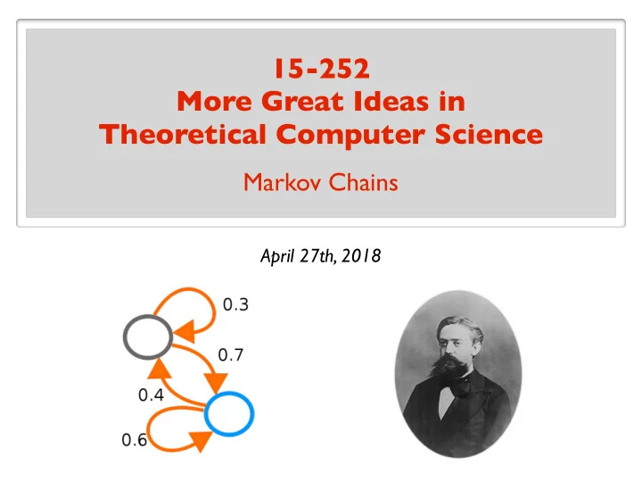
15-252 More Great Ideas in Theoretical Computer Science

Markov Chains

April 27th, 2018

Markov Chain Andrey Markov (1856 - 1922) Russian mathematician. Famous for his work on random processes. A model for the evolution of a random system. The future is independent of the past, given the present.

Pr[X ≥ c · E[X]] ≤ 1/c

( is Markov’s Inequality.)

Cool things about Markov Chains

• It is a very general and natural model.

Applications in: computer science, mathematics, biology, physics, chemistry, economics, psychology, music, baseball,...

• The model is simple and neat.
• Cilantro

The plan

Motivating examples and applications Basic mathematical representation and properties A bit more on applications

The future is independent of the past, given the present.

Some Examples of Markov Chains

Example: Drunkard Walk

Home

Example: Diffusion Process

Example: Weather

A very(!!) simplified model for the weather. Pr[sunny to rainy] = 0.1 Pr[sunny to sunny] = 0.9 Pr[rainy to rainy] = 0.5 Pr[rainy to sunny] = 0.5 Probabilities on a daily basis: Encode more information about current state for a more accurate model.

0.9 0.1 0.5 0.5

• S

R S R S = sunny R = rainy

Example: Life Insurance

Goal of life insurance company: figure out how much to charge the clients. Find a model for how long a client will live. Pr[healthy to sick] = 0.3 Pr[sick to healthy] = 0.8 Pr[sick to death] = 0.1 Pr[healthy to death] = 0.01 Pr[healthy to healthy] = 0.69 Pr[sick to sick] = 0.1 Pr[death to death] = 1 Probabilistic model of health on a monthly basis:

Example: Life Insurance

Goal of life insurance company: figure out how much to charge the clients. Find a model for how long a client will live. Probabilistic model of health on a monthly basis:

0.1 1 0.69

  0.69 0.3 0.01 0.8 0.1 0.1 1  

H S D H S D

Some Applications of Markov Models

Application: Algorithmic Music Composition

Application: Image Segmentation

Application: Automatic Text Generation

“While at a conference a few weeks back, I spent an interesting evening with a grain of salt.” Random text generated by a computer (putting random words together): Google: Mark V Shaney

Application: Speech Recognition

Speech recognition software programs use Markov models to listen to the sound of your voice and convert it into text.

Application: Google PageRank

1997: Web search was horrible Sorts webpages by number of occurrences of keyword(s).

Application: Google PageRank

Founders of Google $40Billionaires Sergey Brin Larry Page

Application: Google PageRank

Jon Kleinberg Nevanlinna Prize

Application: Google PageRank

How does Google order the webpages displayed after a search?

• Reputation of the page.
• Relevance of the page.

2 important factors: Reputation is measured using PageRank. PageRank is calculated using a Markov Chain. The number and reputation of links pointing to that page.

The plan

Motivating examples and applications Basic mathematical representation and properties A bit more on applications

The Setting

1 2 1 2 1 4 3 4 1 1

1 2 3 n Memoryless The next state only depends

• n the current state.

Evolution of the system: random walk on the graph. There is a system with n possible states/values At each time step, the state changes probabilistically. {1, 2, …, n}.

The Definition

The vertices of the graph are called states. The edges are called transitions. The label of an edge is a transition probability.

• At each vertex, the probabilities on outgoing edges

sum to . 1 A Markov Chain is a digraph with

V = {1, 2, . . . , n}

such that:

(We usually assume the graph is strongly connected. i.e. there is a directed path from i to j for any i and j.) self-loops allowed

• Each edge is labeled with a value in

(0, 1]

(a probability).

Define πt[i] = probability of being in state i after exactly t steps.

Notation

Note that someone has to provide . π0 Once this is known, we get the distributions π1, π2, . . . Given some Markov Chain with n states: πt = [p1 p2 · · · pn]

X

i

pi = 1

1 2 n

Notation

   

1 2 1 2

1 1

1 4 3 4

   

1 2 3 4 1 2 3 4 Transition Matrix

1 2 1 2 1 4 3 4 1 1

1 2 3 4 A Markov Chain with n states can be characterized by the n x n transition matrix : K ∀i, j ∈ {1, 2, . . . , n} K[i, j] = Pr[i → j in one step] Note: rows of sum to 1. K

Some Fundamental and Natural Questions

What is the expected time of having visited every state (given some initial state)? What is the expected time of reaching state i when starting at state j ?

. . .

What is the probability of being in state i after t steps (given some initial state)? πt[i] =? How do you answer such questions?

Mathematical representation of the evolution

Suppose we start at state 1 and let the system evolve. How can we mathematically represent the evolution?

1 2 1 2 1 4 3 4 1 1

1 2 3 4

   

1 2 1 2

1 1

1 4 3 4

   

1 2 3 4 1 2 3 4 What is ? π1

⇥1 0⇤

π0 = 1 2 3 4 By inspection, .

= ⇥

1 2 1 2

⇤

π1 1 2 3 4

Mathematical representation of the evolution

   

1 2 1 2

1 1

1 4 3 4

    ⇥1 0⇤

π0

= ⇥

1 2 1 2

⇤

π1 K The probability of states after 1 step:

the new state (probabilistic)

Mathematical representation of the evolution

K The probability of states after 2 steps:

⇥

1 2 1 2

⇤    

1 2 1 2

1 1

1 4 3 4

   

π1

= ⇥

1 8 7 8

⇤

π2

the new state (probabilistic)

Mathematical representation of the evolution

π1 = π0 · K π2 = π1 · K So π2 = (π0 · K) · K = π0 · K2

Mathematical representation of the evolution

In general: If the initial probabilistic state is

⇥p1 p2 · · · pn ⇤ pi = probability of being in state i, p1 + p2 + · · · + pn = 1 ,

after t steps, the probabilistic state is:

⇥p1 p2 · · · pn ⇤

    Transition Matrix    

t

= π0 = πt

i.e., can we say anything about for large ? πt t

Remarkable Property of Markov Chains

Suppose the Markov chain is “aperiodic”. Then, as the system evolves, the probabilistic state converges to a limiting probabilistic state. What happens in the long run? As , for any :

⇥p1 p2 · · · pn ⇤

    Transition Matrix     →

t → ∞

t

π0 = [p1 p2 · · · pn] π

as .

Remarkable Property of Markov Chains

This is unique. π In other words: πt → π t → ∞ stationary/invariant distribution

    Transition Matrix    

π = π Note:

Remarkable Property of Markov Chains

Stationary distribution is . ⇥ 5

6 1 6

⇤ In the long run, it is Sunny 5/6 of the time, it is Rainy 1/6 of the time.

0.9 0.1 0.5 0.5

• ⇥ 5

6 1 6

⇤ = ⇥ 5

6 1 6

⇤

Remarkable Property of Markov Chains

How did I find the stationary distribution?  0.9 0.1 0.5 0.5 2 = 0.86 0.14 0.7 0.3

• 

0.9 0.1 0.5 0.5 4 = 0.8376 0.1624 0.812 0.188

• 

0.9 0.1 0.5 0.5 8 = 0.833443 0.166557 0.832787 0.167213

• Exercise: Why do the rows converge to ?

π

Things to remember

Markov Chains can be characterized by the transition matrix . K What is the probability of being in state i after t steps? πt[i] = (π0 · Kt)[i] πt = π0 · Kt K[i, j] = Pr[i → j in one step]

Things to remember

Theorem (Fundamental Theorem of Markov Chains):

Consider a Markov chain that is strongly connected and aperiodic.

• For any initial distribution ,

π0 lim

t→∞ π0Kt = π

• Let be the number of steps it takes to reach state

provided we start at state . Then,

Tij j i E[Tii] = 1 π[i].

• There is a unique invariant/stationary distriution such that

π π = πK.

The plan

Motivating examples and applications Basic mathematical representation and properties A bit more on applications

How are Markov Chains applied ?

2 common types of applications: Use the Markov chain to simulate the process. e.g. text generation, music composition. e.g. Google PageRank, image segmentation Build a Markov chain as a statistical model of a real-world process. 1. Use a measure associated with a Markov chain to approximate a quantity of interest. 2.

Automatic Text Generation

Generate a superficially real-looking text given a sample document. Idea: From the sample document, create a Markov chain. Use a random walk on the Markov chain to generate text. Example: Collect speeches of Obama, create a Markov chain. Use a random walk to generate new speeches.

Automatic Text Generation

• 1. For each word in the document, create a node/state.
• 2. Put an edge word1 ---> word2

if there is a sentence in which word2 comes after word1.

• 3. Edge probabilities reflect frequency of the pair of

words.

like a the to

like a 3 times like the 4 times like to 2 times

3/9 4/9 2/9

The Markov Chain:

Automatic Text Generation

“I jumped up. I don't know what's going on so I am coming down with a road to opportunity. I believe we can agree on

• r do about the major challenges facing our country.”

Automatic Text Generation

Another use: Build a Markov chain based on speeches of Obama. Build a Markov chain based on speeches of Bush. Given a new quote, can predict if it is by Obama or Bush. (by testing which Markov model the quote fits best)

Google PageRank

The number and reputation of links pointing to you. PageRank is a measure of reputation: The Markov Chain:

Google PageRank

The number and reputation of links pointing to you. PageRank is a measure of reputation: The Markov Chain:

• 1. Every webpage is a node/state.
• 2. Each hyperlink is an edge:

if webpage A has a link to webpage B, A ---> B

• 3a. If A has m outgoing edges, each gets label 1/m.
• 3b. If A has no outgoing edges, put edge A ---> B B

(jump to a random page) ∀

Google PageRank

The stationary probability of A Stationary distribution: probability of being at webpage A in the long run A little tweak: Random surfer jumps to a random page with 15% prob. PageRank of webpage A =

Google PageRank

Google PageRank

Google:

“PageRank continues to be the heart of our software.”

The plan

Motivating examples and applications Basic mathematical representation and properties A bit more on applications