15-251 Great Theoretical Ideas in Computer Science Lecture 2: - - PowerPoint PPT Presentation

Jan 19th, 2017

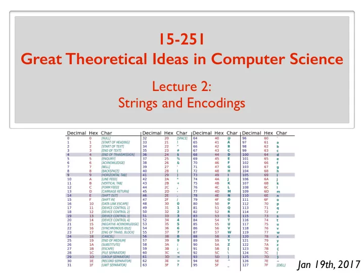
15-251 Great Theoretical Ideas in Computer Science

Lecture 2: Strings and Encodings

Chessboard Puzzle

neighbors in direction N, S, W, E If a square has 2 or more infected neighbors, it becomes infected.

Question: What is the min number of infected squares needed initially to infect the whole board?

Initially, some of the squares are “infected”.

Objects/concepts we want to study and understand Mathematical model (formal, precise definitions) Mathematically/rigorously prove facts/theorems

input data

• utput

data “computer” Computation: manipulation of data. How do we mathematically/formally represent data?

We have already done it for communication purposes. Written communication: 1 2 3 “apple” “car” “happy” “three” or “3”

English alphabet Σ = {a,b,c,d,e,f,g,h,i,j,k,l,m,n,o,p,q,r,s,t,u,v,w,x,y,z} Turkish alphabet Σ = {a,b,c,¸ c,d,e,f,g,¯ g,h,ı,i,j,k,l,m,n,o,¨

• ,p,r,s,¸

s,t,u,¨ u,v,y,z} Binary alphabet Σ = {0, 1} What if we had more symbols? What if we had less symbols?

An element of an alphabet is called a symbol or character. An alphabet is a non-empty, finite set (usually denoted by ). Σ Any (usually finite) sequence of symbols from is called a string (or a word) over . Σ Σ A string is denoted by , where each a1a2a3 . . . an ai ∈ Σ. Example: Some strings over : Σ = {0, 1} ✏ 1 01 1011110101101111 Example: Some strings over : ✏ Σ = {a, b, c} a b c ca caabcccab

Given an alphabet , Σ Σ∗ denotes the set of all finite length strings over . Σ Examples:

{a}∗ = {✏, a, aa, aaa, aaaa, aaaaa, . . .}

{✏, 0, 1, 00, 01, 10, 11, 000, 001, 010, 011, 100, 101, 110, 111 . . .}

{0, 1}∗ =

Length of a string , , is the number of symbols in . s |s| s

Written English

Objects/concepts of interest String encoding

apple Σ = {a,b,c,d,e,f,g,h,i,j,k,l,m,n,o,p,q,r,s,t,u,v,w,x,y,z} car happy Does every string correspond to a valid encoding? Does every object have a corresponding encoding? Can two objects have the same encoding?

Given a set of objects, an encoding of is an injective function A A Enc : A → Σ∗ . Notation: For , denotes a ∈ A hai Enc(a). Technicality Alert: not all sets are encodable.

Examples A = N Σ = {0, 1, 2, 3, 4, 5, 6, 7, 8, 9} Σ = {1} Does affect “encodability”? Σ h36i = “36” Σ = {0, 1} h36i = “100100” h36i = “111111111111111111111111111111111111”

Examples A = Z Σ = {−, 0, 1, 2, 3, 4, 5, 6, 7, 8, 9} Σ = {0, 1} Σ = {1}? h36i = “ 36” h36i = “1100100”

Examples A = N × N Σ = {0, 1} Σ = {0, 1, 2, 3, 4, 5, 6, 7, 8, 9, #} h(3, 36)i = h3, 36i = “3#36” Idea: encode all symbols above using 4 bits (why 4?)

0 → 0000 1 → 0001 2 → 0010 3 → 0011 4 → 0100 5 → 0101 6 → 0110 7 → 0111

8 → 1000 9 → 1001 # → 1010

h3, 36i = “0011101000110110”

Examples A = all undirected graphs 1 4 5 2 3 6 G

“ ” V = {1, 2, 3, 4, 5, 6} E = {{1,2}, {2,3}, {3,4}, {1,4}, {5,6}}

hGi =

Examples A = all undirected graphs 1 4 5 2 3 6         1 1 1 1 1 1 1 1 1 1         1 2 3 4 5 6 1 2 3 4 5 6 G 010100#101000#010100#101000#000001#000010 “ ” hGi =

Examples A = all Python functions def isPrime(N): if (N < 2): return False for factor in range(2, N): if (N % factor == 0): return False return True hisPrimei =

“def isPrime(N):\n if (N < 2):\n return False\n for factor in range(2, N):\n if (N % factor == 0):\n return False\n return True”

Does matter? |Σ| Going from to : |Σ| = k |Σ0| = 2 Σ t encode every symbol of using bits, where . t = dlog2 ke A word of length n

• ver Σ

A word of length

• ver

tn Σ0

Does matter? |Σ| Binary vs Unary 1 2 3 4 5 6 7 8 9 10 11 12 1 10 11 100 101 110 111 1000 1001 1010 1011 1100 1 11 111 1111 11111 111111 1111111 11111111 111111111 1111111111 11111111111 111111111111 ✏

Does matter? |Σ| Binary vs Unary has length in binary blog2 nc + 1 n has length in unary n n has length in base n blogk nc + 1 k Unary is exponentially longer than other bases!

Which sets are encodable? Encodability = Countability (Lecture 7)

What about uncountable sets? Approximate.

Data is represented as finite length strings

• ver some finite alphabet.

Reasoning about computation requires reasoning about strings.

Inductive Reasoning (powerful tool for understanding recursive structures)

Induction Review Domino Principle Line up any number of dominos in a row, knock the first one over and they will all fall.

Induction Review Domino Principle Line up an infinite row of dominoes,

• ne domino for each natural number.

Knock the first one over and they will all fall. Proof: Proof by contradiction: suppose they don’t all fall.

Let k be the lowest numbered domino that remains standing. Domino k-1 did fall. But then k-1 knocks over k, and k falls. So k stands and falls, which is a contradiction.

Induction Review Mathematical induction: statements proved instead of dominoes fallen Infinite sequence of dominoes Infinite sequence of statements: S0, S1, S2, … Fk = “domino k fell” Fk = “Sk proved” Establish:

• 1. F0
• 2. for all k, Fk Fk+1

= ⇒ Conclude: Fk is true for all k.

Induction Review Mathematical induction: statements proved instead of dominoes fallen Infinite sequence of dominoes Infinite sequence of statements: S0, S1, S2, … Fk = “domino k fell” Fk = “Sk proved” Establish:

• 1. F0
• 2. for all k, F0, F1,…,Fk Fk+1

= ⇒ Conclude: Fk is true for all k. “Strong” Induction

Different ways of packaging inductive reasoning Example: Every natural number > 1 can be factored into primes. Proof (by contradiction): Let n be the smallest counter-example. n cannot be prime, so n = ab, where 1 < a, b < n. Since n is the smallest counter-example, a and b must have prime factorizations. Then so does n. Contradiction. “Method of Min Counterexample”

Different ways of packaging induction proofs “Method of Min Counterexample” Let k be the min number such that Sk is not true. Show that Sk’ is not true for k’ < k. Contradiction. By contradiction. The general idea of method of min counterexample:

“Invariant Induction” Example:

At any party, at any point in time, define a person’s parity as odd/even according to the number of hands they have shaken. Statement: number of people of odd parity must be even.

Different ways of packaging induction proofs

“Invariant Induction”

Statement: number of people of odd parity must be even. Initial state: 0 hands have been shaken. 0 people have odd parity. Invariant argument:

• dd
• dd

even even

• dd

even even

• dd

t <— t-2 At an arbitrary point in the party, let t be the number # people with odd parity. t <— t+2 t <— t t <— t parity of t doen’t change. Proof:

Different ways of packaging induction proofs

“Invariant Induction” Time-varying world state: W0, W,1 W2, … Want to prove: statement S is true for all world states. Argue: Statement S is true for W0. If S is true for Wk, it remains true for Wk+1. The general idea of invariant induction: Different ways of packaging induction proofs

“Structural Induction” Induction on objects with a recursive structure. . .

• arrays/lists
• strings
• graphs

. Different ways of packaging induction proofs

“Structural Induction” Recursive definition of a string over : Σ

• the empty sequence is a string.

✏

• if is a string and , then is a string.

x a ∈ Σ ax Different ways of packaging induction proofs

“Structural Induction” Recursive definition of a rooted binary tree:

• a single node r is a binary tree with root r.
• if T1 and T2 are binary trees with roots r1 and r2,

then T which has a node r adjacent to r1 and r2 is a binary tree with root r. T1 T2 T = r1 r2 r

Every node has 0 or 2 children.

Different ways of packaging induction proofs

“Structural Induction” Recursive definition of a rooted binary tree:

• a single node r is a binary tree with root r.
• if T1 and T2 are binary trees with roots r1 and r2,

then T which has a node r adjacent to r1 and r2 is a binary tree with root r. T1 T2 T = r1 r2 r

Every node has 0 or 2 children.

leaves internal nodes

Different ways of packaging induction proofs

“Structural Induction” Example: Let T be a binary tree. Let LT = # leaves in T. Let IT = # internal nodes in T. Then LT = IT + 1. Different ways of packaging induction proofs

“Structural Induction” Proof (by structural induction): T1 T2 T = r1 r2 r Let T be an arbitrary binary tree: We know LT = LT1 + LT2 and IT = IT1 + IT2 + 1. Base case (T is a single node) is true. By IH: LT1 = IT1 + 1 and LT2 = IT2 + 1. So LT = LT1 + LT2 = IT1 + 1 + IT2 + 1 = IT + 1. Different ways of packaging induction proofs

“Structural Induction” The general idea of structural induction:

Base step: check statement true for base case(s) of def’n. Recursive/induction step: prove statement holds for new objects created by the recursive rule, assuming it holds for old objects used in the recursive rule.

Different ways of packaging induction proofs

“Structural Induction” Why is that valid? Follows from strong induction on # of applications

• f the recursive rule to create a particular object.

(even though we don’t phrase it explicitly that way)

Previous example: Could have also packaged it as strong induction on the parameter height.

Different ways of packaging induction proofs

“Structural Induction”

Be careful! What is wrong with the following argument?

Strong induction on height. Base case true. Take an arbitrary binary tree T of height h. Let T’ be the following tree of height h+1: T1 T’ = r r1 r2 blah blah blah Therefore statement true for T’ of height h+1. Different ways of packaging induction proofs

“Structural Induction” Another example with strings: Let be recursively defined as follows: L ⊆ {0, 1}∗

• ;

✏ ∈ L

• if , then .

x, y ∈ L 0x1y0 ∈ L Prove that for any , . w ∈ L #(0, w) = 2 · #(1, w) number of 0’s in w number of 1’s in w Different ways of packaging induction proofs

“Structural Induction” Proof (by structural induction): Base case is and w = ✏ #(0, ✏) = 2 · #(1, ✏). By IH: and #(0, x) = 2 · #(1, x) #(0, y) = 2 · #(1, y). Assume statement is true for all u ∈ L, |u| < k. Let be an arbitrary element of with . w L |w| = k So for some w = 0x1y0 x, y ∈ L, |x| < k, |y| < k. Then: #(0, w) = 2 + #(0, x) + #(0, y) = 2 + 2 · #(1, x) + 2 · #(1, y) = 2(1 + #(1, x) + #(1, y)) = 2 · #(1, w) Different ways of packaging induction proofs

Back to string encodings

input data

• utput

data “computer” What is computation? What is an algorithm? How can we mathematically define them?

First Few Weeks

Can encode/represent any kind of data (numbers, text, pairs of numbers, graphs, images, etc…) with a finite length (binary) string. Seen so far: Before we define algorithm formally, we should define computational problem formally.

An algorithm solves a computational problem. Example description of a computational problem: Given a natural number N, output True if N is prime, and output False otherwise. Example algorithm solving it:

def isPrime(N): if (N < 2): return False for factor in range(2, N): if (N % factor == 0): return False return True

input data

• utput

data

isPrime

Instance Solution No 1 No 2 Yes 3 Yes 4 No . . . . . . 251 Yes . . . . . .

input data

• utput

data

+

Instance Solution 0, 0 0, 1 1 1, 1 2 2, 2 4 2, 3 5 10, 1 11 100, 99 199 . . . . . .

input data

• utput

data

Sorting

[“vanilla”, “mind”, “Anil”, “yogurt”, “doesn’t”] Instance Solution [“Anil”, “doesn’t”, “mind”, “vanilla”, “yogurt”]

A computational problem is a function f : A → B . A = B = set of possible input objects (called instances) set of possible output objects (called solutions) But in TCS, we don’t deal with arbitrary objects, we deal with strings (encodings). f 0 : Σ⇤ → Σ⇤ f : A → B

Enc

Technicality: What if does not correspond to an encoding of an instance? w ∈ Σ∗

f : Σ∗ → Σ∗ Definition: A computational problem is a function . Definition: A decision problem is a function . f : Σ∗ → {0, 1}

No, Yes False, True Reject, Accept

IMPORTANT DEFINITIONS Definition: A subset is called a language. L ⊆ Σ∗

IMPORTANT RELATIONSHIP There is a one-to-one correspondence between decision problems and languages.

Instance Solution ✏ 1 1 1 1 00 1 01 10 11 1 000 1 001 . . . . . .

L ⊆ Σ∗ {✏, 0, 1, 00, 11, 000, . . .} L =

Our focus will be on languages! (decision problems)

• Convenient restriction.
• Usually “without loss of generality”.

(more on this next lecture)

Are all languages computable/decidable? How can we prove that a language is not decidable? How do we measure complexity of algorithms deciding languages? P = NP? How do we classify languages according to resources needed to decide them? INTERESTING QUESTIONS WE WILL EXPLORE ABOUT COMPUTATION