13 symbolic mt 2 weighted finite state transducers
play

13 Symbolic MT 2: Weighted Finite State Transducers The previous - PDF document

13 Symbolic MT 2: Weighted Finite State Transducers The previous section introduced a number of word-based translation models, their parameter estimation methods, and their application to alignment. However, it intentionally glossed over an


  1. 13 Symbolic MT 2: Weighted Finite State Transducers The previous section introduced a number of word-based translation models, their parameter estimation methods, and their application to alignment. However, it intentionally glossed over an important question: how to generate translations from them. This section introduces a general framework for expressing our models graphs: weighted finite-state transducers . It explains how to encode a simple translation model within this framework and how this allows us to perform search. 13.1 Graphs and the Viterbi Algorithm 
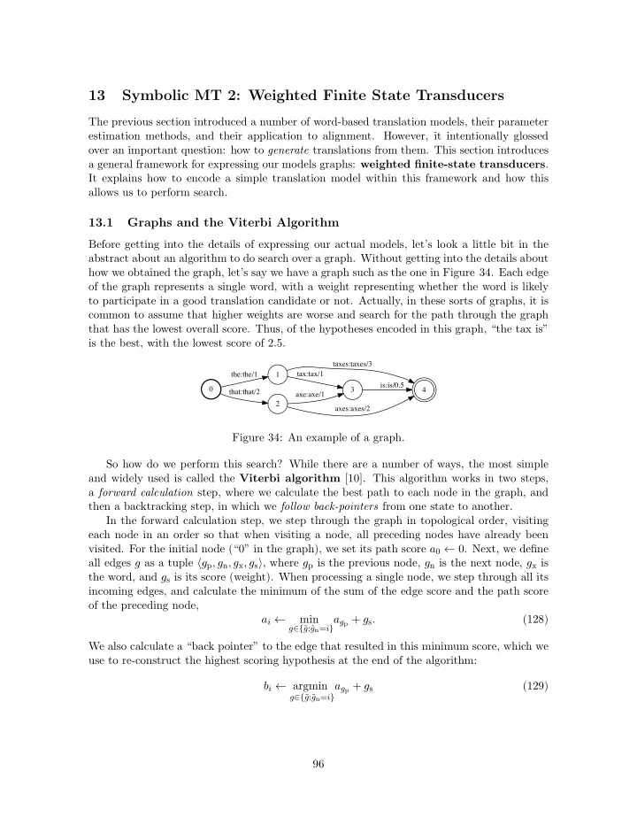
Before getting into the details of expressing our actual models, let’s look a little bit in the abstract about an algorithm to do search over a graph. Without getting into the details about how we obtained the graph, let’s say we have a graph such as the one in Figure 34. Each edge of the graph represents a single word, with a weight representing whether the word is likely to participate in a good translation candidate or not. Actually, in these sorts of graphs, it is common to assume that higher weights are worse and search for the path through the graph that has the lowest overall score. Thus, of the hypotheses encoded in this graph, “the tax is” is the best, with the lowest score of 2.5. taxes:taxes/3 tax:tax/1 the:the/1 1 is:is/0.5 0 3 4 that:that/2 axe:axe/1 2 axes:axes/2 Figure 34: An example of a graph. So how do we perform this search? While there are a number of ways, the most simple and widely used is called the Viterbi algorithm [10]. This algorithm works in two steps, a forward calculation step, where we calculate the best path to each node in the graph, and then a backtracking step, in which we follow back-pointers from one state to another. In the forward calculation step, we step through the graph in topological order, visiting each node in an order so that when visiting a node, all preceding nodes have already been visited. For the initial node (“0” in the graph), we set its path score a 0 0. Next, we define all edges g as a tuple h g p , g n , g x , g s i , where g p is the previous node, g n is the next node, g x is the word, and g s is its score (weight). When processing a single node, we step through all its incoming edges, and calculate the minimum of the sum of the edge score and the path score of the preceding node, a i min g n = i } a g p + g s . (128) g ∈ { ˜ g ;˜ We also calculate a “back pointer” to the edge that resulted in this minimum score, which we use to re-construct the highest scoring hypothesis at the end of the algorithm: b i argmin a g p + g s (129) g ∈ { ˜ g ;˜ g n = i } 96

  2. In the example above, the calculation would be equal to: a 1 = a 0 + g the,s = 0 + 1 = 1 b 1 = g the a 2 = a 0 + g that,s = 0 + 2 = 2 b 2 = g that a 3 = min ( a 1 + g tax,s , a 2 + g axe,s ) = min (1 + 1 , 2 + 1) = 2 b 3 = g tax a 4 = min ( a 1 + g taxes,s , a 2 + g axes,s , a 3 + g is,s ) = min (1 + 3 , 2 + 3 , 2 + 0 . 5) = 2 . 5 b 4 = g is The next step is the back-pointer following step. In this step, we start at the final state (“4” in the example), and iterate over the back-pointers g p of each edge, one by one. First, we observe b 4 , note the word g is , x is “is”, then step to g is , p = 3. We continue to follow b 3 , note the word “tax”, step to b 1 , note the word “the”, step to b 0 and terminate because we’ve reached the beginning of the sentence. This leaves us with the words “is tax the”, which we then reverse to obtain “the tax is”, our highest scoring hypothesis. 13.2 Weighted Finite State Automata and A Language Model This sort of graph where g = h g p , g n , g x , g s i is also called a weighted finite state automaton (WFSA). These WFSAs can be used to express a wide variety of strings and their weightings over them, 41 and being able to think about various tasks in this way opens up possibilities for doing a wide variety of processing in a single framework. The following explanation describes some basic properties of WFSAs, and interested readers can reference [7] for a comprehensive explanation. One example of something that can be expressed as an WFSA is the smoothed n -gram languages models described in Section 3. Let’s say that we have a 2-gram language model interpolated according to Equation 9 over the set of words “she”, “i”, “ate”, “an”, “a”, “apple”, “peach”, “apricot” calculated from the following corpus: she ate an apple she ate a peach i ate an apricot (130) We also assume that the interpolation coe ffi cient is ↵ = 0 . 1. 41 Specifically, they are able to express all regular languages , with a weight assigned to each string contained therein. 97

  3. Given this, we will have two classes of probabilities, one where the bigram count is non- zero, such as P (apple | an), which (sparing the details) becomes the probability: P ( e t = apple | e t − 1 = an) = (1 � ↵ ) P ML ( e t = apple | e t − 1 = an) + ↵ P ML ( e t = apple) = 0 . 91 2 + 0 . 1 1 15 = 0 . 456 . We also have probabilities where where the bigram count is zero, these are essentially equal to the unigram probability discounted by ↵ . For example: P ( e t = apple | e t − 1 = a) = (1 � ↵ ) P ML ( e t = apple | e t − 1 = a) + ↵ P ML ( e t = apple) = 0 + 0 . 1 1 15 = 0 . 006 </s>/1.6094 apricot/2.7081 <eps>/2.3026 apricot </s>/0.0834 apricot/0.7838 <eps>/2.3026 </s>/0 </s>/0.0834 an apple/0.7838 an/2.0149 apple/2.7081 apple an/0.4888 </s>/0.0834 <eps>/2.3026 <eps>/2.3026 i ate/0.0834 NULL i/2.7081 <eps>/2.3026 ate/1.6094 i/1.182 <eps>/2.3026 ate <s> she/2.0149 ate/0.0834 a/1.182 she/0.4888 she <eps>/2.3026 <eps>/2.3026 peach peach/0.098 <eps>/2.3026 a a/2.7081 peach/2.7081 Figure 35: A 2-gram language model as a WFSA. Edge labels are “word/score”, where the score is represented as a negative log probability. States are labeled with the context e t − 1 that the represent, where “NULL” represents unigrams. “ h eps i ” represents an ✏ edge, which can be used to fall back from the unigram state to the bigram state. The way we express this in a WFSA is shown in Figure 35. Each state label indicates the bigram context, so the state labeled “an” will represent probabilities P ( e t | e t − 1 = an). Edges outgoing from a labeled state (with an edge label that is not “ h eps i ”, which we will get to later), represent negative log bigram probabilities. So for example, P ( e t = apple | e t − 1 = an) = 0 . 456, which indicates that the edge outgoing from the state “an” that is labeled with 98

  4. “apple” will have an edge weight of � log P ( e t = apple | e t − 1 = an) ⇡ 0 . 7838. We also have a state labeled “NULL”, which represents all unigram probabilities P ( e t ). All outgoing edges here represent a unigram probability. Now, to the h eps i edges, which are called ✏ edges or ✏ transitions. ✏ edges are basically edges that we can follow at any time, without consuming a token in the input sequence. In the case of language models, these transitions are used to express the fact that sometimes we won’t have a transition that we can match for a particular context, and will instead want to fall back to a more general context using interpolation. For example, after “an” we may see the word “peach” and want to calculate its probability. In this case, we would fall back from the “an” state to the “NULL” state using the ✏ edge, which incurs a score of � log ↵ = 2 . 3026, then follow the edge from the “NULL” state to the “peach” state, resulting in a probability of � log P ( e t = peach) = 2 . 7081. Of course, we could also create an edge directly from “an” to “peach” with a probability � log ↵ P ( e t = peach), but by using the ✏ edges we are able to avoid explicitly enumerating all pairs of words, improving our memory e ffi ciency while obtaining the exact same results. 13.3 Weighted Finite State Transducers and a Translation Model As could be seen from the previous section, WFSAs are able to express sets of strings with corresponding scores over them. This is enough for when we want to express something like a language model, but what if we want to express a translation model that takes in a string and translates it into another string? This sort of string transduction can be done with another formalism called weighted finite state transducers (WFSTs). WFSTs are essentially similar to WFSAs with an addition symbol output g y , leading to g = h g p , g n , g x , g y , g s i . Thus, each edge takes in a symbol, outputs another symbol, and gives a score to this particular transduction. To give a very simple example, let’s assume a translation model that is even simpler than IBM Model 1: one that calculates P ( F | E ) by taking one e t at a time and independently calculates the translation probability of the corresponding word f t | E | Y P ( F | E ) = P ( f t | e t ) . (131) t =1 Assume that we have the following Spanish corpus equivalent to our English corpus in Equa- tion 130: 42 ella comi´ o una manzana ella comi´ o un melocot´ on yo comi un albaricoque (132) In this case, we can learn translation probabilities for each word, for example: P ( f = ella | e = she) = 1 (133) 42 Spanish allows dropping of the pronoun “yo” – equivalent to “i” – and a natural translation would probably do so. But for the sake of simplicity, let’s leave it in to maintain the one-to-one relationship with the English words, and we’ll deal with the problem of translations that are not one-to-one in a bit. 99

Download Presentation
Download Policy: The content available on the website is offered to you 'AS IS' for your personal information and use only. It cannot be commercialized, licensed, or distributed on other websites without prior consent from the author. To download a presentation, simply click this link. If you encounter any difficulties during the download process, it's possible that the publisher has removed the file from their server.

Recommend


More recommend