SLIDE 1 1
ECO 300 – Fall 2005 – November 22
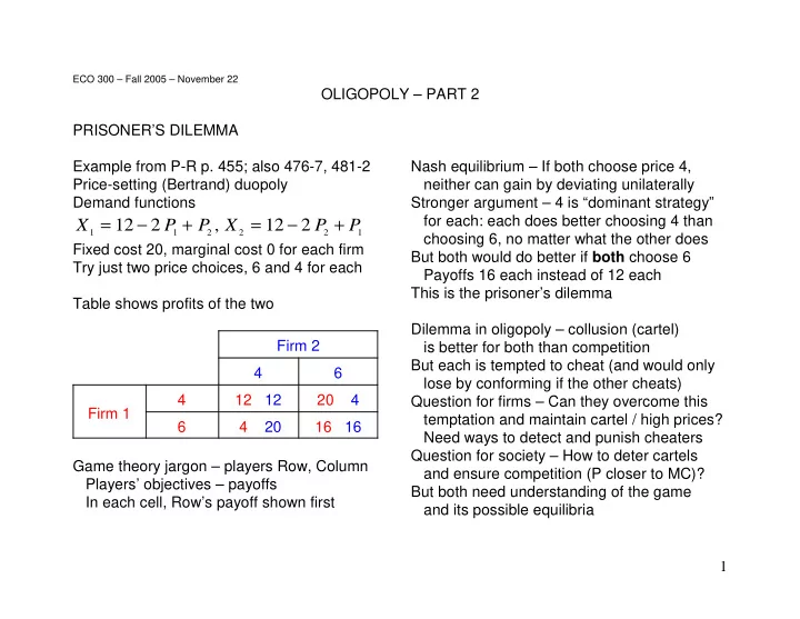
OLIGOPOLY – PART 2 PRISONER’S DILEMMA Example from P-R p. 455; also 476-7, 481-2 Price-setting (Bertrand) duopoly Demand functions
X P P X P P
1 1 2 2 2 1
12 2 12 2 = − + = − + ,
Fixed cost 20, marginal cost 0 for each firm Try just two price choices, 6 and 4 for each Table shows profits of the two Firm 2 4 6 Firm 1 4 12 12 20 4 6 4 20 16 16 Game theory jargon – players Row, Column Players’ objectives – payoffs In each cell, Row’s payoff shown first Nash equilibrium – If both choose price 4, neither can gain by deviating unilaterally Stronger argument – 4 is “dominant strategy” for each: each does better choosing 4 than choosing 6, no matter what the other does But both would do better if both choose 6 Payoffs 16 each instead of 12 each This is the prisoner’s dilemma Dilemma in oligopoly – collusion (cartel) is better for both than competition But each is tempted to cheat (and would only lose by conforming if the other cheats) Question for firms – Can they overcome this temptation and maintain cartel / high prices? Need ways to detect and punish cheaters Question for society – How to deter cartels and ensure competition (P closer to MC)? But both need understanding of the game and its possible equilibria
SLIDE 2
2 REPEATED INTERACTION (P-R pp. 484-8) Above game played each period. From one period to the next, payoffs grow at rate g, and money values are discounted at the interest rate r Also, probability p that for some outside reason, interaction will discontinue Tacit collusion can be sustained by various strategies that make it costly to cheat. Simplest example here: “Grim trigger strategies” – both start by playing the collusive actions, but if anyone ever cheats, the collusion collapses in all future periods and the game is thereafter played to its competitive or dilemma equilibrium Cheater gains 20 - 16 = 4 in one period, but loses (opportunity sense) 16 - 12 = 4 ever after The future loss has expected present discounted value
4 1 1 1 4 1 1 1 2 4 1 1 1 3 41 ( )( ) ( )( ) ( )( ) − + + + − + + ⎡ ⎣ ⎢ ⎤ ⎦ ⎥ + − + + ⎡ ⎣ ⎢ ⎤ ⎦ ⎥ + = − p g r p g r p g r k k L
where k = (1-p)(1+g)/(1+r) . Example: If p = 0.2, g = 0.05, r = 0.1, then k = 0.76, RHS = 12.1 > 4 But if p = 0.4, g = – 0.02, r = 0.2, then k = 0.49, RHS = 3.84 < 4 So collusion more likely if [1] interest rate r at which future money flows are discounted is low, [2] interaction is likely to persist (low p), [3] industry is growing or stable (high g) All these are conditions ensuring that the future is important relative to the present Implicit in this – length of the period. Interpretation – how long it takes to detect cheating Therefore speed and accuracy of cheating important for successful cartelization In practice, firms’ demands and costs are asymmetric. Price wars are more costly for large firms, so small firms may hope to get away with cheating P-R pp. 457-67 for other practical issues – signaling collusive price and allocating market shares as demand and cost conditions change, deterring or responding to outside competition, ...
SLIDE 3 3 ENTRY DETERRENCE (P-R pp. 491-502, specific example from p. 497-8) Existing firm (incumbent) trying to deter potential entrant by threat – Says “I will charge low price (start a price war) if you enter” Problem – threat may not be credible; potential entrant may believe that if it comes in and puts the matter to the test, the incumbent will back off and accommodate the new firm Game “tree” shown on right. Consists of “nodes” and “branches” Each node shows the player who takes action there; emerging branches are available actions At final or terminal nodes, show resulting “payoffs” if that path is followed in play of game Asterisks show the optimal action of each player at each node With these numbers, if Entrant chooses In, Incumbent’s optimal strategy is High Price Therefore threat of price war is not credible Equilibrium of game found by rollback: Start at last decision nodes and work back Find optimal choice at each node, looking ahead and folding in all optimal choices at later nodes Resulting path of play - continuous sequence
- f asterisks from the initial to a final node
Incumbent would like to make threat credible One method – install (sink) capacity ahead of time, enough to meet demand at the low price
SLIDE 4
4 The extra capacity costs 50 If high price is charged, quantity is low, capacity goes unused, but its cost is sunk Profits lower than if capacity was not sunk If low price is charged, capacity is used. Profits no different than non-sunk case where the same capacity would have to be acquired later to meet demand at the low price Bigger game tree with new initial node for incumbent’s capacity choice Lower half same as old tree In upper half, if entrant In, Low price becomes optimal for incumbent – threat of price war becomes credible In rollback equilibrium play Incumbent instals capacity Entrant stays Out Incumbent prices High Excess capacity stays idle Incumbent’s profit 150 (200 monopoly - 50 capacity cost) Not as good as 200, but better than the 130 that comes without the capacity strategy that makes threat credible Other paths to credibility – reputation in repeated play, irrationality, ...
SLIDE 5 5 STACKELBERG LEADERSHIP (P-R pp. 447-8, 452) Quantity-setting as in Cournot, but firm 1 moves first, firm 2 moves second Numbers as in November 17 Oligopoly handout; pp. 3-4 Firm 2's reaction curve is Q2 = 75 - 0.75 Q1 ; this will be its choice at its second move Firm 1 will recognize this, so at its first move will choose Q1 to maximize its profit
( )
Π1
1 2 1 1 1 1 1 1 1 1
200 100 200 75 0 75 100 25 0 25 2 = − − − = − − + − = − ( ) ( . ) . Q Q Q Q Q Q Q Q Q Q
To maximize this, , or Q1 = 50
d dQ Q Π1
1 1
25 05 / . = − =
Have not drawn game tree, but this is rollback equilibrium of the sequential-move game Then can solve for other magnitudes. Table shows comparison Type of oligopoly Q1 Q2 P
B1 B2
Cournot 20 60 120 400 2400 Stackelberg (firm 1 leads) 50 37.5 112.5 625 937.5 Quantity-leadership is better for firm 1 and for society than simultaneous play. Reason – by increasing Q1 above its Cournot level, firm 1 can get firm 2 to produce less Q2 But firm 2'a backing off is less than 1-for-1, so total Q increases, P decreases closer to MC So consumers gain. Total industry profit declines, but firm 1 gains at the expense of firm 2 With price-setting, leadership is often disadvantageous when products are substitutes – the other firm moving second can see your price and then just undercut you
SLIDE 6
6 MONOPOLISTIC COMPETITION (P-R pp. 436-41) Case where several firms sell close but not perfect substitutes Free entry / exit yields (approximately) zero profit for each firm Examples – many consumer products, supermarkets in large town, global auto industry? Multi-firm model of location differentiation. Consider n firms along a circle of circumference L Each firm has fixed cost F and constant marginal cost c If firm charges P, effective price at distance x is P + k x Consider symmetric equilibrium where each firm charges price P* (more complex cases exist) Left figure shows circle with 8 firms; right, just 3 neighbors, with prices and effective prices If one firm deviates to charge P, it sells to distance x either side, defined by P + k x = P* + k ( L/n – x ) , or x = L/(2n) + (P*-P) / (2k) So total quantity it sells is Q = 2 x = L/n + (P*-P)/k
SLIDE 7
7 This firm’s profit Π =
− − = − + − ⎡ ⎣ ⎢ ⎤ ⎦ ⎥ − ( ) ( ) * P c Q F P c L n P P k F
This firm treats others’ P* as given, and chooses P to maximize its own profit
∂ ∂ Π P L n P P k P c k = + − ⎡ ⎣ ⎢ ⎤ ⎦ ⎥ − − = * ( ) 1
We want a symmetric equilibrium where P = P*, so (P-c) / k = L / n, or P = c + k L / n Then each firm sells to x = L/(2n) either side of its location, for total quantity Q = L/n Profit of each firm is B = (P-c) Q – F = k (L/n)2 – F Entry / exit will reduce this to zero, so k (L/n)2 = F, or n = L /(k/F) More firms if [1] larger market, [2] lower fixed cost, [3] larger disutility cost of non-ideal product Equilibrium can be illustrated in figure on right similar to P-R p. 438 Fig. 12.1 (b) except that here MC is horizontal For one firm, P = P*, Q = L/n is optimal because its MR = MC there Its maximized profit is zero because AR = AC there So fixed cost F must equal profit rectangle (P*–MC) (L/n)