11 { < t (0), t (1), t ( n -1)> Correct Concept: Learn a decent - PDF document
Learning Theory Theorems that characterize classes of learning problems or specific algorithms in terms of computational complexity or sample complexity , i.e. the number of training examples CS 391L: Machine Learning: necessary or
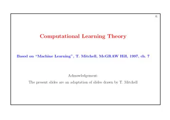
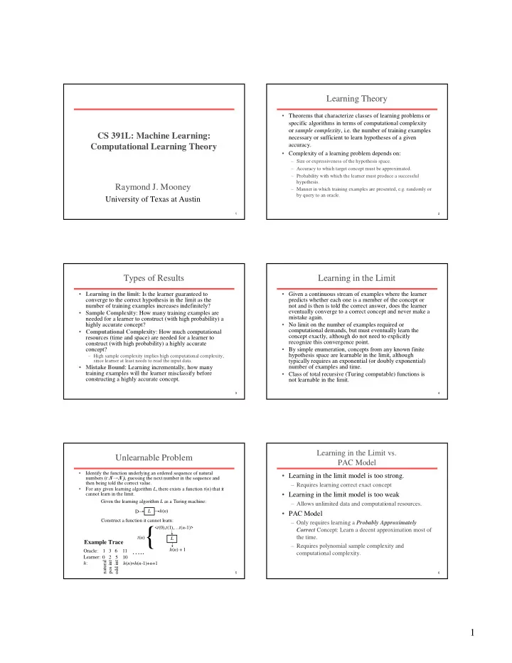
Learning Theory • Theorems that characterize classes of learning problems or specific algorithms in terms of computational complexity or sample complexity , i.e. the number of training examples CS 391L: Machine Learning: necessary or sufficient to learn hypotheses of a given Computational Learning Theory accuracy. • Complexity of a learning problem depends on: – Size or expressiveness of the hypothesis space. – Accuracy to which target concept must be approximated. – Probability with which the learner must produce a successful hypothesis. Raymond J. Mooney – Manner in which training examples are presented, e.g. randomly or by query to an oracle. University of Texas at Austin 1 2 Types of Results Learning in the Limit • Learning in the limit : Is the learner guaranteed to • Given a continuous stream of examples where the learner converge to the correct hypothesis in the limit as the predicts whether each one is a member of the concept or number of training examples increases indefinitely? not and is then is told the correct answer, does the learner • Sample Complexity : How many training examples are eventually converge to a correct concept and never make a mistake again. needed for a learner to construct (with high probability) a highly accurate concept? • No limit on the number of examples required or • Computational Complexity : How much computational computational demands, but must eventually learn the concept exactly, although do not need to explicitly resources (time and space) are needed for a learner to recognize this convergence point. construct (with high probability) a highly accurate concept? • By simple enumeration, concepts from any known finite hypothesis space are learnable in the limit, although – High sample complexity implies high computational complexity, since learner at least needs to read the input data. typically requires an exponential (or doubly exponential) • Mistake Bound : Learning incrementally, how many number of examples and time. training examples will the learner misclassify before • Class of total recursive (Turing computable) functions is constructing a highly accurate concept. not learnable in the limit. 3 4 Learning in the Limit vs. Unlearnable Problem PAC Model • Identify the function underlying an ordered sequence of natural • Learning in the limit model is too strong. numbers ( t : N → N) , guessing the next number in the sequence and then being told the correct value. – Requires learning correct exact concept For any given learning algorithm L , there exists a function t ( n ) that it • cannot learn in the limit. • Learning in the limit model is too weak Given the learning algorithm L as a Turing machine: – Allows unlimited data and computational resources. L h ( n ) D • PAC Model Construct a function it cannot learn: – Only requires learning a Probably Approximately 11 { < t (0), t (1),… t ( n -1)> Correct Concept: Learn a decent approximation most of t ( n ) the time. L Example Trace – Requires polynomial sample complexity and h ( n ) + 1 Oracle: 1 3 6 ….. computational complexity. Learner: 0 2 5 10 natural odd int h : pos int h ( n )= h ( n -1)+ n +1 5 6 1
Cannot Learn Exact Concepts Cannot Learn Even Approximate Concepts from Limited Data, Only Approximations from Pathological Training Sets Positive Positive Classifier Classifier Learner Learner Negative Negative Positive Negative Positive Negative 7 8 PAC Learning Formal Definition of PAC-Learnable • Consider a concept class C defined over an instance space • The only reasonable expectation of a learner X containing instances of length n , and a learner, L , using a hypothesis space, H . C is said to be PAC-learnable by L is that with high probability it learns a close using H iff for all c ∈ C , distributions D over X , 0< ε <0.5, approximation to the target concept. 0< δ <0.5; learner L by sampling random examples from distribution D , will with probability at least 1 − δ output a • In the PAC model, we specify two small hypothesis h ∈ H such that error D (h) ≤ ε , in time polynomial in 1/ ε , 1/ δ , n and size( c ). parameters, ε and δ , and require that with • Example: probability at least (1 − δ ) a system learn a – X: instances described by n binary features – C: conjunctive descriptions over these features concept with error at most ε . – H : conjunctive descriptions over these features – L : most-specific conjunctive generalization algorithm (Find-S) – size(c) : the number of literals in c (i.e. length of the conjunction). 9 10 Issues of PAC Learnability Consistent Learners • A learner L using a hypothesis H and training data • The computational limitation also imposes a polynomial constraint on the training set size, D is said to be a consistent learner if it always since a learner can process at most polynomial outputs a hypothesis with zero error on D data in polynomial time. whenever H contains such a hypothesis. • How to prove PAC learnability: • By definition, a consistent learner must produce a – First prove sample complexity of learning C using H is hypothesis in the version space for H given D . polynomial. – Second prove that the learner can train on a • Therefore, to bound the number of examples polynomial-sized data set in polynomial time. needed by a consistent learner, we just need to • To be PAC-learnable, there must be a hypothesis bound the number of examples needed to ensure in H with arbitrarily small error for every concept that the version-space contains no hypotheses with in C , generally C ⊆ H. unacceptably high error. 11 12 2
ε -Exhausted Version Space Proof • Let H bad ={ h 1 ,… h k } be the subset of H with error > ε . The VS • The version space, VS H , D , is said to be ε -exhausted iff every hypothesis in it has true error less than or equal to ε . is not ε -exhausted if any of these are consistent with all m • In other words, there are enough training examples to examples. guarantee than any consistent hypothesis has error at most ε . • A single h i ∈ H bad is consistent with one example with • One can never be sure that the version-space is ε -exhausted, probability: ≤ − ε but one can bound the probability that it is not. P h i e ( consist ( , )) ( 1 ) j • Theorem 7.1 (Haussler, 1988): If the hypothesis space H is • A single h i ∈ H bad is consistent with all m independent random finite, and D is a sequence of m ≥ 1 independent random examples for some target concept c , then for any 0 ≤ ε ≤ 1, examples with probability: P h i D ≤ − ε m the probability that the version space VS H , D is not ε - ( consist ( , )) ( 1 ) exhausted is less than or equal to: • The probability that any h i ∈ H bad is consistent with all m | H | e – ε m examples is: P H D = P h D ∨ ∨ h D ( consist ( , )) ( consist ( , ) consist ( , )) bad k 1 L 13 14 Proof (cont.) Sample Complexity Analysis • Since the probability of a disjunction of events is at most • Let δ be an upper bound on the probability of not the sum of the probabilities of the individual events: exhausting the version space. So: ≤ − ε m ≤ δ P H D ≤ H − ε m P H D H e ( consist ( , )) ( consist ( , )) ( 1 ) bad bad bad δ e − ε m ≤ H • Since: | H bad | ≤ | H | and (1– ε ) m ≤ e – ε m , 0 ≤ ε ≤ 1, m ≥ 0 δ − ε m ≤ ln( ) ≤ − ε m P H D H e ( consist ( , )) H bad δ ≥ − ε Q.E.D m ln / (flip inequality ) H H ≥ ε m ln / δ 1 ≥ + ε m H ln ln / δ 15 16 Sample Complexity Result Sample Complexity of Conjunction Learning Consider conjunctions over n boolean features. There are 3 n of these • • Therefore, any consistent learner, given at least: since each feature can appear positively, appear negatively, or not 1 appear in a given conjunction. Therefore |H|= 3 n, so a sufficient + H ε ln ln / δ number of examples to learn a PAC concept is: 1 1 examples will produce a result that is PAC. + n ε = + n ε ln ln 3 / ln ln 3 / δ δ • Just need to determine the size of a hypothesis space to • Concrete examples: instantiate this result for learning specific classes of – δ = ε =0.05, n =10 gives 280 examples concepts. – δ =0.01, ε =0.05, n =10 gives 312 examples • This gives a sufficient number of examples for PAC – δ = ε =0.01, n =10 gives 1,560 examples learning, but not a necessary number. Several – δ = ε =0.01, n =50 gives 5,954 examples approximations like that used to bound the probability of a • Result holds for any consistent learner, including FindS. disjunction make this a gross over-estimate in practice. 17 18 3
Recommend
More recommend
Explore More Topics
Stay informed with curated content and fresh updates.
