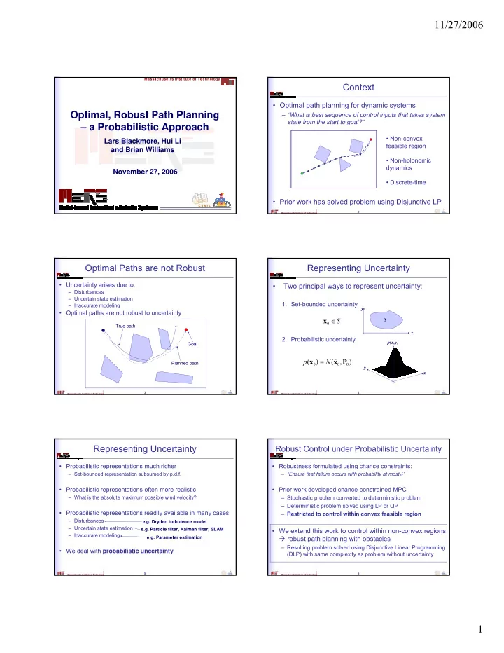
11/27/2006 Massachusetts Institute of Technology Context Optimal - - PDF document

SLIDE 1

11/27/2006 1

November 27, 2006

Massachusetts Institute of Technology

Optimal, Robust Path Planning – a Probabilistic Approach

Lars Blackmore, Hui Li and Brian Williams

2

Context

• Optimal path planning for dynamic systems

– “What is best sequence of control inputs that takes system state from the start to goal?”

• Prior work has solved problem using Disjunctive LP
• Non-convex

feasible region

• Non-holonomic

dynamics

• Discrete-time

3

Optimal Paths are not Robust

• Uncertainty arises due to:

– Disturbances – Uncertain state estimation – Inaccurate modeling

• Optimal paths are not robust to uncertainty

Planned path True path Goal

4

Representing Uncertainty

• Two principal ways to represent uncertainty:
• 1. Set-bounded uncertainty
• 2. Probabilistic uncertainty

S ∈ x

x y S

) , ˆ ( ) ( P x x N p =

x y p(x,y)

5

Representing Uncertainty

• Probabilistic representations much richer

– Set-bounded representation subsumed by p.d.f.

• Probabilistic representations often more realistic

– What is the absolute maximum possible wind velocity?

• Probabilistic representations readily available in many cases

– Disturbances – Uncertain state estimation – Inaccurate modeling

• We deal with probabilistic uncertainty

e.g. Parameter estimation e.g. Dryden turbulence model e.g. Particle filter, Kalman filter, SLAM

6

Robust Control under Probabilistic Uncertainty

• Robustness formulated using chance constraints:

– “Ensure that failure occurs with probability at most δ”

• Prior work developed chance-constrained MPC

– Stochastic problem converted to deterministic problem – Deterministic problem solved using LP or QP – Restricted to control within convex feasible region

• We extend this work to control within non-convex regions

robust path planning with obstacles

– Resulting problem solved using Disjunctive Linear Programming (DLP) with same complexity as problem without uncertainty

SLIDE 2

11/27/2006 2

7

Problem Statement

• Design a finite, optimal sequence of control

inputs u0…uk-1 such that the expected final vehicle position is the goal

– Take into account uncertainty such that collision with any obstacle at a given time step occurs with probability at most δ

8

Problem Statement

p(failure) ≤ δ Expected path Expected final position

9

Technical Approach: Assumptions

• Assume discrete-time linear stochastic system:
• Assume that and are known.
• Initial state x0 is unknown, but assume p(x0) is known
• Polytopic obstacles
• All uncertainty is Gaussian

t t t t t

w Bu Ax x ν + + + =

+1 Noise due to disturbances Noise due to uncertain model

) (

t

w p ) (

t

p ν

10

Technical Approach: Summary

• 1. Convert stochastic problem into deterministic one
• 2. Show that deterministic problem can be solved

using Disjunctive Linear Programming

11

Linear Chance Constraints

• Consider linear chance constraint on an uncertain

multivariate variable X:

• Probability of constraint violation depends on:
• 1. Covariance of X
• 2. Distance of E[X] from constraint

b Ax =

] [X E

Covariance ellipse of X

" ) ( " δ ≤ > b Ax p

x b Ax

b Ax

d X p p

∫

>

= > ) ( ) (

12

Linear Chance Constraints

• So for given covariance P, linear chance constraint is

equivalent to deterministic linear constraint on E[X]

b Ax =

∆

⇔ ≤ > ) ( δ b Ax p ∆ − ≤ b x A ] [ E

Ensure mean at least distance ∆ from constraint to guarantee chance constraint satisfied

SLIDE 3

11/27/2006 3

13

Linear Chance Constraints

• How is ∆ calculated?
• Find vector normal to constraint line
• The distribution of projected along is a

univariate Gaussian with variance

• So ∆ can be calculated using a simple lookup of erf,

the Gaussian c.d.f. function

x n ˆ b Ax = n ˆ n P n ˆ ˆ T ∆

14

Obstacle Chance Constraints

• Extension: use this to ensure that an obstacle is hit with

probability at most δ

• Notice that:

p(collision with obstacle) ≤ p(constraint violated)

• Simply need to ensure that expected state is ∆ away from at

least one of obstacle’s constraints

– Conservatism introduced

S T

ij ij

b x A =

Obstacle i Constraint j

x x d X p d X p

T S S

∫ ∫

∪

≤ ) ( ) (

15

Multiple Obstacles

• Must ensure that probability of hitting any obstacle

is at most δ

– Probabilities of collision are not mutually exclusive

p(collision with obstacle 1 or 2) = p(collision w. obs. 1) + p(collision w. obs. 2)

– But can bound probability of collision with any obstacle

p(collision with obstacle 1 or 2) ≤ p(collision w. obs. 1) + p(collision w. obs. 2)

• Constrain probability of hitting each of N obstacles

to be at most δ/N

– Then probability of collision with any obstacle guaranteed to be at most δ – Additional conservatism introduced

LB2

16

Robust Path Planning as DLP

• Important analytic properties:

– Future state distribution is Gaussian – Future state mean is linear function of control inputs – Future state covariance is not a function of control inputs

• Hence the constraint:

“Ensure expected state is ∆ away from at least one of obstacle’s constraints” – is a disjunctive linear constraint on control inputs u1…t

• Cost functions such as fuel use can be expressed as

piecewise linear functions of control inputs Problem can be posed as a Disjunctive Linear Program

17

Robust Path Planning as DLP

• Summary:

– Calculate covariance Pt of predicted state at each t in horizon – Calculate required margin ∆t for each t in horizon to ensure probability of failure less than δ – Pose disjunctive linear program to ensure margin satisfied – Solve using efficient, readily available solvers

1

∑

=

=

T i i

J u minimize subject to

t ij t ij i

] E[X ∆ − ≤ ∨ b A

j t

• bstacle

each and step each time for

18

Results

• Trade off performance against plan conservatism

2 4 6 8 10 12 14 16 2 4 6 8 10 12 14 x(meters) y(meters) No uncertainty ∆ = 0.1 ∆ = 0.001 ∆ = 0.0001 10

−5

10

−4

10

−3

10

−2

10

−1

60 65 70 75 80 85 90 95 100 105 110 Maximum Probability of Collision (∆) Fuel Use

SLIDE 4

Slide 15 LB2 Work out how to link into the next slide - see next slide

Lars Blackmore, 6/10/2006

SLIDE 5

11/27/2006 4

19

Conclusion

• Robust path planning problem can be solved as DLP

– Essentially same complexity as DLP that does not take into account uncertainty (one lookup, matrix multiplication per constraint)

• The catch?

– The resulting plan is excessively conservative

• We guarantee p(collision) is less than δ, but in practice, p(collision) is

much less than δ

• Hence there exists a better solution that still satisfies chance constraint
• If we try to constrain the probability of collision at any time step, we get

very conservative plans

• Solution: Ongoing research
• 1. Particle Control approach approximates distributions using samples
• Approximate approach instead of conservative approach
• 2. Ellipsoidal approximations have been used in the literature to solve

analogous problems

20

Questions?

21

Backup

• Conservatism plot