11 1 ant algorithms
play

11.1 Ant Algorithms Dorigo et al. (1991 onwards), Hoos & Sttzle - PowerPoint PPT Presentation

T79.4201 Search Problems and Algorithms T79.4201 Search Problems and Algorithms 11.1 Ant Algorithms Dorigo et al. (1991 onwards), Hoos & Sttzle (1997), ... Inspired by experiment of real ants selecting the shorter of two paths


  1. T–79.4201 Search Problems and Algorithms T–79.4201 Search Problems and Algorithms 11.1 Ant Algorithms 
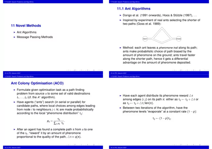
◮ Dorigo et al. (1991 onwards), Hoos & Stützle (1997), ... ◮ Inspired by experiment of real ants selecting the shorter of two paths (Goss et al. 1989): 11 Novel Methods ◮ Ant Algorithms ◮ Message Passing Methods NEST FOOD ◮ Method: each ant leaves a pheromone trail along its path; ants make probabilistic choice of path biased by the amount of pheromone on the ground; ants travel faster along the shorter path, hence it gets a differential advantage on the amount of pheromone deposited. I.N. & P .O. Autumn 2007 I.N. & P .O. Autumn 2007 T–79.4201 Search Problems and Algorithms T–79.4201 Search Problems and Algorithms Ant Colony Optimisation (ACO) ◮ Formulate given optimisation task as a path finding problem from source s to some set of valid destinations ◮ Have each agent distribute its pheromone reward △ τ t 1 ,..., t n (cf. the A ∗ algorithm). among edges ( i , j ) on its path π : either as τ ij ← τ ij + △ τ or ◮ Have agents (“ants”) search (in serial or parallel) for as τ ij ← τ ij + △ τ / len ( π ) . candidate paths, where local choices among edges leading ◮ Between two iterations of the algorithm, have the from node i to neighbours j ∈ N i are made probabilistically pheromone levels “evaporate” at a constant rate ( 1 − ρ ) : according to the local “pheromone distribution” τ ij : τ ij ← ( 1 − ρ ) τ ij . τ ij p ij = . ∑ j ∈ N i τ ij ◮ After an agent has found a complete path π from s to one of the t k , “reward” it by an amount of pheromone proportional to the quality of the path, △ τ ∝ q ( π ) . I.N. & P .O. Autumn 2007 I.N. & P .O. Autumn 2007

  2. T–79.4201 Search Problems and Algorithms T–79.4201 Search Problems and Algorithms ACO motivation ACO variants ◮ Local choices leading to several good global results get Several modifications proposed in the literature: reinforced by pheromone accumulation. ◮ To exploit best solutions, allow only best agent of each ◮ Evaporation of pheromone maintains diversity of search. iteration to distribute pheromone. (I.e. hopefully prevents it getting stuck at bad local minima.) ◮ To maintain diversity, set lower and upper limits on the ◮ Good aspects of the method: can be distributed; adapts edge pheromone levels. automatically to online changes in the quality function q ( π ) . ◮ To speed up discovery of good paths, run some local ◮ Good results claimed for Travelling Salesman Problem, optimisation algorithm on the paths found by the agents. Quadratic Assignment, Vehicle Routing, Adaptive Network ◮ Etc. Routing etc. I.N. & P .O. Autumn 2007 I.N. & P .O. Autumn 2007 T–79.4201 Search Problems and Algorithms T–79.4201 Search Problems and Algorithms An ACO algorithm for the TSP (2/2) An ACO algorithm for the TSP (1/2) ◮ The local choice of moving from city i to city j is biased ◮ Dorigo et al. (1991) according to weights: ◮ At the start of each iteration, m ants are positioned at τ α ij ( 1 / d ij ) β random start cities. a ij = ∑ j ∈ N i τ α ◮ Each ant constructs probabilistically a Hamiltonian tour π ij ( 1 / d ij ) β , on the graph, biased by the existing pheromone levels. where α , β ≥ 0 are parameters controlling the balance (NB. the ants need to remember and exclude the cities between the current strength of the pheromone trail τ ij vs. they have visited during the search.) the actual intercity distance d ij . ◮ In most variations of the algorithm, the tours π are still ◮ Thus, the local choice distribution at city i is: locally optimised using e.g. the Lin-Kernighan 3-opt procedure. a ij p ij = , ◮ The pheromone award for a tour π of length d ( π ) is ∑ j ∈ N ′ i a ij △ τ = 1 / d ( π ) , and this is added to each edge of the tour: where N ′ i is the set of permissible neighbours of i after τ ij ← τ ij + 1 / d ( π ) . cities visited earlier in the tour have been excluded. I.N. & P .O. Autumn 2007 I.N. & P .O. Autumn 2007

  3. T–79.4201 Search Problems and Algorithms T–79.4201 Search Problems and Algorithms 11.2 Message Passing Methods Belief Propagation (or the Sum-Product Algorithm ): Survey Propagation ◮ Pearl (1986) and Lauritzen & Spiegelhalter (1986). ◮ Braunstein, Mézard & Zecchina (2005). ◮ Originally developed for probabilistic inference in graphical ◮ Refinement of Belief Propagation to dealing with models; specifically for computing marginal distributions of “clustered” solution spaces. free variables conditioned on determined ones. ◮ Based on statistical mechanics ideas of the structure of ◮ Recently generalised to many other applications by configuration spaces near a “critical point”. Kschischang et al. (2001) and others. ◮ Remarkable success in solving very large “hard” randomly ◮ Unifies many other, independently developed important generated Satisfiability instances. algorithms: Expectation-Maximisation (statistics), Viterbi ◮ Success on structured problem instances not so clear. and “Turbo” decoding (coding theory), Kalman filters (signal processing), etc. ◮ Presently of great interest as a search heuristic in constraint satisfaction. I.N. & P .O. Autumn 2007 I.N. & P .O. Autumn 2007 T–79.4201 Search Problems and Algorithms T–79.4201 Search Problems and Algorithms Belief propagation Bias-guided search ◮ Method is applicable to any constraint satisfaction problem, If the biases β i could be computed effectively, they could be but for simplicity let us focus on Satisfiability. used e.g. as a heuristic to guide backtrack search: ◮ Consider cnf formula F determined by variables x 1 ,..., x n and clauses C 1 ,..., C m . Represent truth values as function BPSearch( F : cnf): ξ ∈ { 0 , 1 } . if F has no free variables then return val ( F ) ∈ { 0 , 1 } ◮ Denote the set of satisfying truth assignments for F as else ¯ β ← BPSurvey( F ); S = { x ∈ { 0 , 1 } n | C 1 ( x ) = ··· = C m ( x ) = 1 } . choose variable x i for which β i ( ξ ) = max ; ◮ We aim to estimate for each variable x i and truth value val ← BPSearch( F [ x i ← ξ ] ); ξ ∈ { 0 , 1 } the bias of x i towards ξ in S : if val = 1 then return 1 else return BPSearch( F [ x i ← ( 1 − ξ )] ); β i ( ξ ) = Pr x ∈ S ( x i = ξ ) . end if . ◮ If for some x i and ξ , β i ( ξ ) ≈ 1 , then x i is a “backbone” Alternately, the bias values could be used to determine variable variable for the solution space, i.e. most solutions x ∈ S share the feature that x i = ξ . flip probabilities in some local search method etc. I.N. & P .O. Autumn 2007 I.N. & P .O. Autumn 2007

  4. T–79.4201 Search Problems and Algorithms T–79.4201 Search Problems and Algorithms Message passing on factor graphs A factor graph ◮ The problem of course is that the biases are in general Factor graph representation of formula difficult to compute. (It is already NP-complete to F = ( x 1 ∨ x 2 ) ∧ ( ¯ x 2 ∨ x 3 ) ∧ ( ¯ x 1 ∨ ¯ x 3 ) : determine whether S � = / 0 in the first place.) ◮ Thus, the BP survey algorithm aims at just estimating the a b c biases by iterated local computations (“message passing”) on the factor graph structure determined by formula F . ◮ The factor graph of F is a bipartite graph with nodes 1 , 2 ,... corresponding to the variables and nodes a , b ,... corresponding to the clauses. An edge connects nodes i and u if and only if variable x i occurs in clause C u (either 3 1 2 as a positive or a negative literal). I.N. & P .O. Autumn 2007 I.N. & P .O. Autumn 2007 T–79.4201 Search Problems and Algorithms T–79.4201 Search Problems and Algorithms Propagation rules ◮ Initially, all the variable-to-clause messages are initialised Belief messages to µ i → a ( ξ ) = 1 / 2 . ◮ Then beliefs are propagated in the network according to ◮ The BP survey algorithm works by iteratively exchanging the following update rules, until no more changes occur (a “belief messages” between interconnected variable and fixpoint of the equations is reached): clause nodes. ∏ ◮ The variable-to-clause messages µ i → a ( ξ ) represent the µ b → i ( ξ ) “belief” (approximate probability) that variable x i would b ∈ N i \ a µ i → a ( ξ ) = µ b → i ( ξ )+ ∏ ∏ µ b → i ( 1 − ξ ) have value ξ in a satisfying assignment, if it was not influenced by clause C a . b ∈ N i \ a b ∈ N i \ a µ a → i ( ξ ) = ∑ C a ( x ) · ∏ µ j → a ( x j ) ◮ The clause-to-variable messages µ a → i ( ξ ) represent the x : x i = ξ j ∈ N a \ i belief that clause C a can be satisfied, if variable x i is assigned value ξ . (Here notation N u \ v means the neighbourhood of node u , excluding node v .) ◮ Eventually the variable biases are estimated as β i ( ξ ) ≈ µ i → a ( ξ ) . I.N. & P .O. Autumn 2007 I.N. & P .O. Autumn 2007

Download Presentation
Download Policy: The content available on the website is offered to you 'AS IS' for your personal information and use only. It cannot be commercialized, licensed, or distributed on other websites without prior consent from the author. To download a presentation, simply click this link. If you encounter any difficulties during the download process, it's possible that the publisher has removed the file from their server.

Recommend


More recommend