10/5/2009 Outline Scalable Network Distance Browsing in Spatial - PDF document

10/5/2009 Outline Scalable Network Distance Browsing in Spatial � Introduction to Spatial Networks and Network Databases Distances - Hanan Samet, Jagan Sankaranarayanan, Houman � Conventional Algorithms for Nearest Neighbor Alborzi, SIGMOD ‘08 Queries in SNDB � Shortest-Path Quadtrees By: By: � Morton Blocks Nakul Desai � Distance Encoding � Best-first k NN algorithm � Execution and space requirements � Experimental Results � Conclusion � References Contd… 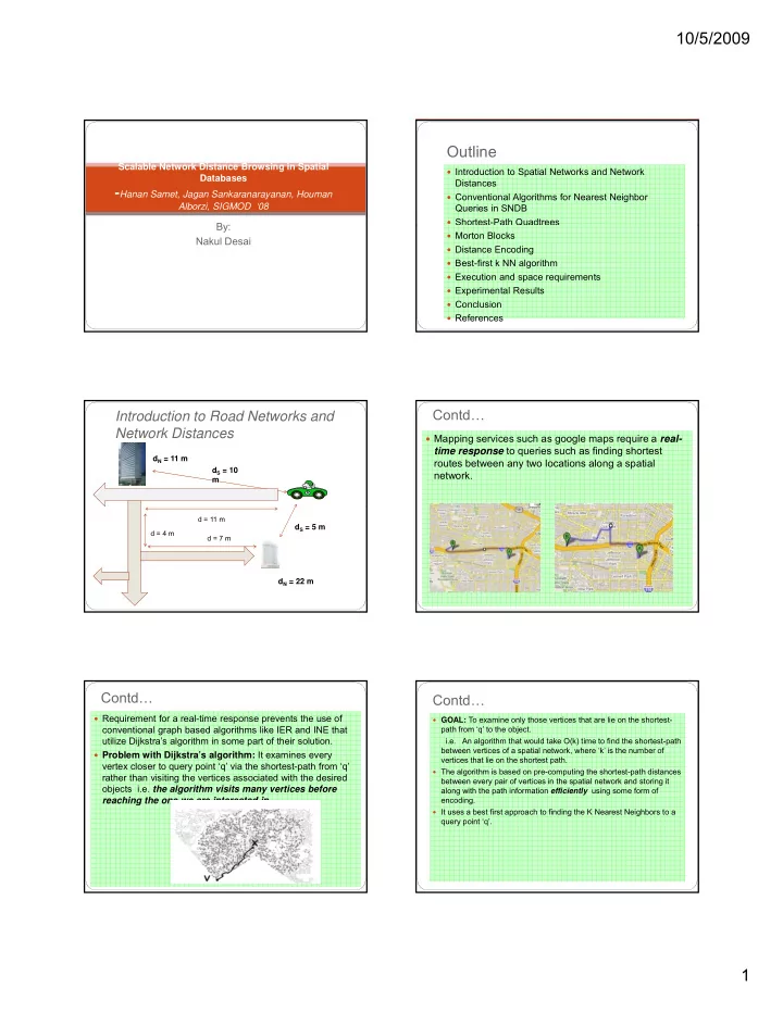Introduction to Road Networks and Network Distances � Mapping services such as google maps require a real- time response to queries such as finding shortest d N = 11 m routes between any two locations along a spatial d S = 10 network. m d = 11 m d S = 5 m d = 4 m d = 7 m d N = 22 m Contd… Contd… � Requirement for a real-time response prevents the use of � GOAL: To examine only those vertices that are lie on the shortest- conventional graph based algorithms like IER and INE that path from ‘q’ to the object. utilize Dijkstra’s algorithm in some part of their solution. i.e. An algorithm that would take O(k) time to find the shortest-path between vertices of a spatial network, where ‘k’ is the number of � Problem with Dijkstra’s algorithm: It examines every vertices that lie on the shortest path. vertex closer to query point ‘q’ via the shortest-path from ‘q’ � The algorithm is based on pre-computing the shortest-path distances rather than visiting the vertices associated with the desired between every pair of vertices in the spatial network and storing it objects i.e. the algorithm visits many vertices before bj t i th l ith i it ti b f along with the path information efficiently using some form of reaching the one we are interested in. encoding. � It uses a best first approach to finding the K Nearest Neighbors to a query point ‘q’. 1

10/5/2009 IER (Incremental Euclidean Restriction) � Based on the fact that d S (q, v) ≤ d N (q, v). i.e the Euclidean distance lower bounds the Network Distance . � First retrieve the Euclidean NN ‘v1’ to ‘q’ using the R-tree based NN algorithm. v1 � Compute the Network Distance ‘d N (q, v1)’ using Dijkstra’s algorithm. d S Due to the Euclidean Lower Bound Property, objects closer to q than v1 � (q,v2) must lie within the Euclidean distance d SMAX = d N (q,v1) i.e in the shaded q d N (q,v2) region. v2 v2 v1 d S (q,v1) d SMax = d N (q,v2) v3 q d N (q,v1) • Since d N (q,v2) < d N (q,v1), v2 becomes the current NN and d SMAX is updated accordingly. • The next Euclidean NN ‘v3’ falls out of the shaded region i.e its d S (q,v3) > d N d SMax = d N (q,v1) (q,v2), the algorithm terminates with v2 as the NN. • This can be extended to k NN accordingly by considering d SMAX = d N (q,vk), where vk is the kth Euclidean NN of q. Representing shortest path information Representing shortest path information � Using Adjacency Lists: � Drawbacks of Adjacency Lists: Adj (u) = { (v1,v2,v3) , (v4,v5) , (v6,v7,v8,v9) , … } Absence of index Searches are sequencial Space Requirement for each List is O(N). � Solution Shortest path Map w1 w2 w3 v4 v4 v3 v3 w2 v5 w2 v5 v1 v1 u u v2 v2 w3 w3 w1 w1 v6 v6 v8 v8 v9 v9 v7 v7 • Each element of the Adjacency List has some spatial coherence in the sense that • The advantage of grouping vertices on the basis of the regions in which they lie they are in close spatial proximity. and identifying each region by the first vertex on the shortest-path into it from • Thus each element can be viewed as a region ‘r i ‘ corresponding to a vertex ‘w i ‘ to vertex ‘u’ is that we can now make use of point location operations to determine the which ‘u’ is connected by means of an edge ‘e i ‘. region that contains the destination vertex. • We can now replace the adjacency list by a map corresponding to the vertex ‘u’ • We can now find the shortest path to a group of vertices. termed as the shortest-path map. • The regions can now be index based on a spatial index structure such as the region Quadtree. Region • Can we use R-trees ? R2 v4 v3 w2 v1 v5 u v2 w3 Region w1 v6 R1 v8 Region v9 R3 v7 2

10/5/2009 Shortest Path Quadtree Morton Blocks • A Morton Block is an Integer representing a Quadtree block. 1) Color-coding the map • It is based on the Morton Order or the Z-Order, which is a space filling curve that 2) Store the regions in a region Quadtree that visits all the points in 2-D space exactly once in a predetermined order. 3) Represent the regions by a Morton Block • A mapping from 2-D space to a 1-D space of Integers. v4 v3 v5 w2 v1 u v2 w3 w1 v6 v8 v9 v7 • A link and a distance interval are associated with each morton block. • The procedure to form morton blocks is as below: Procedure Mortonize[u, T] Input: u є V , T is a Region Quadtree on V Output: MortonList: list of Morton blocks with associated links and distance intervals 1. MortonList � empty 2. for each leaf-block ‘b’ є T visited in Morton-order do 3. if all points v in b are of same color then 4. append b to MortonList 5. else 6. recursively split b until S, the resultant set of blocks, is single colored 6 recursively split b until S the resultant set of blocks is single colored 7. merge S with MortonList 8. while Morton blocks can be merged do 9. merge sibling blocks if of the same color 10. for each Morton block b є MortonList do 11. λ ‐‐ = Minimum ratio of the network distance (d N (u,v)) to the spatial distance (d S (u,v)) from u to all the destination vertices in morton block b 12. λ + = Maximum ratio of the network distance (d N (u,v)) to the spatial distance (d S (u,v)) from u to all the destination vertices in morton block b 13.Associate ( λ ‐‐ , λ + ) with b 14.Return Morton list. Retrieving the Shortest Path Distance Encoding • Given a source vertex ‘s’ , a destination vertex ‘d’, the next link ‘t’ in the Most spatial applications require an approximate estimate of the distance shortest path between s and d is obtained by performing a simple binary between two vertices u and v on a spatial network. search for a morton block containing d from the morton list. • Since each morton block for a vertex s is associated with a link, λ – d S (u,v) ≤ d N (u,v) ≤ λ + d S (u,v) t � b.link • Now t is the next link after s in the shortest path between s and v. Since λ – and λ + are associated with a morton block ‘b’ , given vertices u and v • The above algorithm is repeated until v is obtained. an initial Interval d N (u,v) is made available for the shortest path distance • dist = dist + d N (s,t) between u and v. Block b • The shortest path between s and d requires exactly k steps, where, 2 2 k = |No of vertices in the shortest path between s and d | 2 λ – d S (u,v) = 15 7 λ + d S (u,v) = 21 5 10 3