1 Variance of 6 Sided Die Properties of Variance Var(aX + b) = a 2 - - PDF document

1
SMART_READER_LITE
LIVE PREVIEW

1 Variance of 6 Sided Die Properties of Variance Var(aX + b) = a 2 - - PDF document

Welcome to St. Petersburg! Breaking Vegas Game set-up Consider even money bet (e.g., bet Red in roulette) We have a fair coin (come up heads with p = 0.5) p = 18/38 you win $Y, otherwise (1 p) you lose $Y Let n =


slide-1
SLIDE 1

1 Welcome to St. Petersburg!

  • Game set-up
  • We have a fair coin (come up “heads” with p = 0.5)
  • Let n = number of coin flips before first “tails”
  • You win $2n
  • How much would you pay to play?
  • Solution
  • Let X = your winnings
  • E[X] =
  • I’ll let you play for $1 million... but just once! Takers?

  

                                  

1 3 4 2 3 1 2 1

2 2 1 ... 2 2 1 2 2 1 2 2 1 2 2 1

i i i

  

 0 2

1

i

Breaking Vegas

  • Consider even money bet (e.g., bet “Red” in roulette)
  • p = 18/38 you win $Y, otherwise (1 – p) you lose $Y
  • Consider this algorithm for one series of bets:

1. Y = $1 2. Bet Y 3. If Win, stop 4. if Loss, Y = 2 * Y, goto 2

  • Let Z = winnings upon stopping
  • E[Z]
  • Expected winnings ≥ 0. Use algorithm infinitely often!

... ) 1 2 4 ( 38 18 38 20 ) 1 2 ( 38 18 38 20 1 38 18

2

                                     1 38 20 1 1 38 18 38 20 38 18 2 2 38 18 38 20

1 1

                                           

  

      i i i j j i i i

Vegas Breaks You

  • Why doesn’t everyone do this?
  • Real games have maximum bet amounts
  • You have finite money
  • Not be able to keep doubling bet beyond certain point
  • Casinos can kick you out
  • But, if you had:
  • No betting limits, and
  • Infinite money, and
  • Could play as often as you want...
  • Then, go for it!
  • And tell me which planet you are living on

Variance

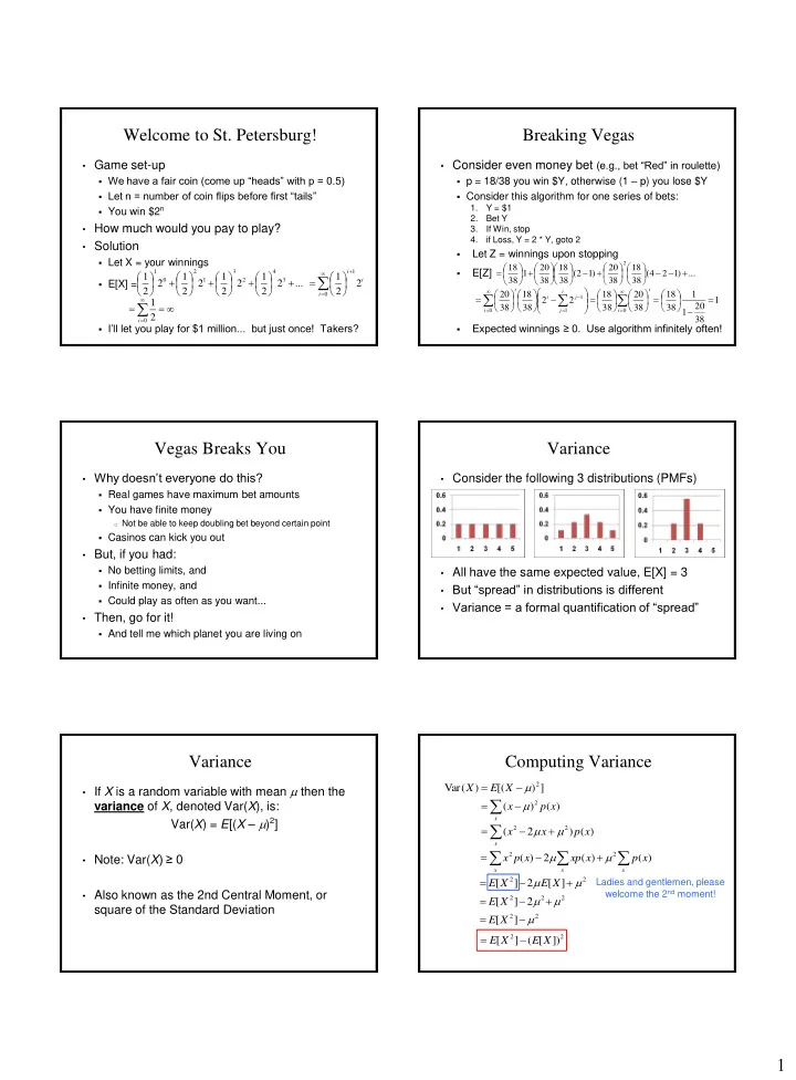
  • Consider the following 3 distributions (PMFs)
  • All have the same expected value, E[X] = 3
  • But “spread” in distributions is different
  • Variance = a formal quantification of “spread”

Variance

  • If X is a random variable with mean m then the

variance of X, denoted Var(X), is: Var(X) = E[(X – m)2]

  • Note: Var(X) ≥ 0
  • Also known as the 2nd Central Moment, or

square of the Standard Deviation

Computing Variance

] ) [( ) ( Var

2

m   X E X

 

x

x p x ) ( ) (

2

m

  

x

x p x x ) ( ) 2 (

2 2

m m

  

  

x x x

x p x xp x p x ) ( ) ( 2 ) (

2 2

m m

2 2

] [ 2 ] [ m m    X E X E

2 2 2

2 ] [ m m    X E

2 2]

[ m   X E

2 2

]) [ ( ] [ X E X E  

Ladies and gentlemen, please welcome the 2nd moment!

slide-2
SLIDE 2

2 Variance of 6 Sided Die

  • Let X = value on roll of 6 sided die
  • Recall that E[X] = 7/2
  • Compute E[X2]

           

6 91 6 1 6 6 1 5 6 1 4 6 1 3 6 1 2 6 1 1 ] [

2 2 2 2 2 2 2

       X E

2 2

]) [ ( ] [ ) ( Var X E X E X   12 35 2 7 6 91

2

        

Properties of Variance

  • Var(aX + b) = a2Var(X)
  • Proof:

Var(aX + b) = E[(aX + b)2] – (E[aX + b])2 = E[a2X2 + 2abX + b2] – (aE[X] + b)2 = a2E[X2] + 2abE[X] + b2 – (a2(E[X])2 + 2abE[X] + b2) = a2E[X2] – a2(E[X])2 = a2(E[X2] – (E[X])2) = a2Var(X)

  • Standard Deviation of X, denoted SD(X), is:
  • Var(X) is in units of X2
  • SD(X) is in same units as X

) ( Var ) ( SD X X 

Jacob Bernoulli

  • Jacob Bernoulli (1654-1705), also known as

“James”, was a Swiss mathematician

  • One of many mathematicians in Bernoulli family
  • The Bernoulli Random Variable is named for him
  • He is my academic great11-grandfather
  • Resemblance to Charlie Sheen weak at best

Bernoulli Random Variable

  • Experiment results in “Success” or “Failure”
  • X is random indicator variable (1 = success, 0 = failure)
  • P(X = 1) = p(1) = p

P(X = 0) = p(0) = 1 – p

  • X is a Bernoulli Random Variable: X ~ Ber(p)
  • E[X] = p
  • Var(X) = p(1 – p)
  • Examples
  • coin flip
  • random binary digit
  • whether a disk drive crashed

Binomial Random Variable

  • Consider n independent trials of Ber(p) rand. var.
  • X is number of successes in n trials
  • X is a Binomial Random Variable: X ~ Bin(n, p)
  • By Binomial Theorem, we know that
  • Examples
  • # of heads in n coin flips
  • # of 1’s in randomly generated length n bit string
  • # of disk drives crashed in 1000 computer cluster
  • Assuming disks crash independently

n i p p i n i p i X P

i n i

,..., 1 , ) 1 ( ) ( ) (             

1 ) (  

  i

i X P

Three Coin Flips

  • Three fair (“heads” with p = 0.5) coins are flipped
  • X is number of heads
  • X ~ Bin(3, 0.5)

8 1 ) 1 ( 3 ) (

3

            p p X P 8 3 ) 1 ( 2 3 ) 2 (

1 2

            p p X P 8 3 ) 1 ( 1 3 ) 1 (

2 1

            p p X P 8 1 ) 1 ( 3 3 ) 3 (

3

            p p X P

slide-3
SLIDE 3

3 Error Correcting Codes

  • Error correcting codes
  • Have original 4 bit string to send over network
  • Add 3 “parity” bits, and send 7 bits total
  • Each bit independently corrupted (flipped) in transition

with probability 0.1

  • X = number of bits corrupted: X ~ Bin(7, 0.1)
  • But, parity bits allow us to correct at most 1 bit error
  • P(a correctable message is received)?
  • P(X = 0) + P(X = 1)

Error Correcting Codes (cont)

  • Using error correcting codes: X ~ Bin(7, 0.1)
  • P(X = 0) + P(X = 1) = 0.8503
  • What if we didn’t use error correcting codes?
  • X ~ Bin(4, 0.1)
  • P(correct message received) = P(X = 0)
  • Using error correction improves reliability ~30%!

4783 . ) 9 . ( ) 1 . ( 7 ) (

7

           X P 3720 . ) 9 . ( ) 1 . ( 1 7 ) 1 (

6 1

           X P 6561 . ) 9 . ( ) 1 . ( 4 ) (

4

           X P

Genetic Inheritance

  • Person has 2 genes for trait (eye color)
  • Child receives 1 gene (equally likely) from each parent
  • Child has brown eyes if either (or both) genes brown
  • Child only has blue eyes if both genes blue
  • Brown is “dominant” (d) , Blue is recessive (r)
  • Parents each have 1 brown and 1 blue gene
  • 4 children, what is P(3 children with brown eyes)?
  • Child has blue eyes: p = (½) (½) = ¼ (2 blue genes)
  • P(child has brown eyes) = 1 – (¼) = 0.75
  • X = # of children with brown eyes. X ~ Bin(4, 0.75)

4219 . ) 25 . ( ) 75 . ( 3 4 ) 3 (

1 3

           X P

Properties of Bin(n, p)

  • We have X ~ Bin(n, p)
  • Noting that:
  • Set k = 1  E[X] = np
  • Set k = 2  E[X2] = npE[Y + 1] = np[(n – 1)p + 1]
  • Var(X) = np[(n – 1)p + 1] – (np)2 = np(1 – p)
  • Note: Ber(p) = Bin(1, p)

i n i n i k i n i n i k k

p p i n i p p i n i X E

   

                   

 

) 1 ( ) 1 ( ] [

1

1 where , ) 1 ( 1 ) 1 ( ) 1 ( 1 1 ] [

) 1 ( 1 1 1 1 1

                         

        

 

j i p p j n j np p p i n i np X E

j n j n j k i n i n i k k

                           1 1 ))! 1 ( ) 1 (( )! 1 ( )! 1 ( )! ( ! ! i n n i n i n n i n i n i i n i

) , 1 ( ~ where ], ) 1 [(

1

p n Bin Y Y npE

k

  

PMF for X ~ Bin(10, 0.5)

k P(X=k)

PMF for X ~ Bin(10, 0.3)

k P(X=k)

slide-4
SLIDE 4

4 Power of Your Vote

  • Is it better to vote in small or large state?
  • Small: more likely your vote changes outcome
  • Large: larger outcome (electoral votes) if state swings
  • a (= 2n) voters equally likely to vote for either candidate
  • You are deciding (a + 1)st vote
  • Use Stirling’s Approximation:
  • Power = P(tie) * Elec. Votes =
  • Larger state = more power

n n n

n n n n n n P

2

2 ! ! )! 2 ( 2 1 2 1 2 ) tie voters 2 (                      

 2 !

2 / 1 n n

e n n

 

    n e n e n n P

n n n n n

1 2 2 2 ) 2 ( ) tie voters 2 (

2 2 1 2 2 2 / 1 2

 

   

  a c ac a 2 ) ( ) 2 / ( 1 