PERCOLATION WITHOUT FKG VINCENT BEFFARA AND DAMIEN GAYET Abstract. - - PDF document

percolation without fkg
SMART_READER_LITE
LIVE PREVIEW

PERCOLATION WITHOUT FKG VINCENT BEFFARA AND DAMIEN GAYET Abstract. - - PDF document

PERCOLATION WITHOUT FKG VINCENT BEFFARA AND DAMIEN GAYET Abstract. We prove a Russo-Seymour-Welsh theorem for large and natural perturbative families of discrete percolation models that do not necessarily satisfy the Fortuin-Kasteleyn- Ginibre


slide-1
SLIDE 1

PERCOLATION WITHOUT FKG

VINCENT BEFFARA AND DAMIEN GAYET

  • Abstract. We prove a Russo-Seymour-Welsh theorem for large and natural perturbative

families of discrete percolation models that do not necessarily satisfy the Fortuin-Kasteleyn- Ginibre condition of positive association. In particular, we prove the box-crossing property for the antiferromagnetic Ising model with small parameter, and for certain discrete Gaussian fields with oscillating correlation function. R´ esum´

  • e. Nous d´

emontrons un th´ eor` eme de type Russo-Seymour-Welsh pour des familles na- turelles de mod` eles de percolation discr` ete, qui ne satisfont pas n´ ecessairement la condition de corr´ elation positive de Fortuin-Kasteleyn-Ginibre. Nos m´ ethodes s’appliquent en particulier au mod` ele d’Ising antiferromagn´ etique ` a haute temp´ erature et ` a certains champs gaussiens discrets dont la fonction de corr´ elation n’est pas de signe constant.

The antiferromagnetic Ising model, with a (percolating) component highlighted

Keywords: Percolation, Ising model, negative association. Mathematics subject classification 2010: 60K35, 60G15, 82B20

Date: September 21, 2018.

1

slide-2
SLIDE 2

2 VINCENT BEFFARA AND DAMIEN GAYET

Contents 1. Introduction 2 1.1. The setting 3 1.2. Topological definitions 4 1.3. Gaussian fields 6 1.4. The Ising model. 6 1.5. Open questions. 7 2. Proof of the main result 7 2.1. Well behaved processes 8 2.2. Ideas of the proof of Theorem 2.7 10 2.3. Topological preliminaries 10 2.4. Finite-range models 13 2.5. General models 24 3. Applications 26 3.1. Discrete Gaussian fields 26 3.2. The Ising model 28 Appendix A. A smoothed random wave model. 30 References 31

  • 1. Introduction

The Fortuin-Kasteleyn-Ginibre condition (FKG for short) is a crucial tool in the study

  • f percolation and the ferromagnetic Ising model. It states that two increasing events are

positively correlated, which allows for instance to construct the pure phases of the Ising model

  • r to build percolation crossings of long rectangles from more elementary blocks, typically

crossings of squares; it is an essential tool in much of the literature in statistical mechanics. For Bernoulli percolation, it was first observed by Harris [10]; in the case of the sign of a Gaussian field, it was proved by Pitt [13] that if the correlation function is positive, then the FKG condition is satisfied. The property was essential in our previous paper [1], where we proved that continuous, positively correlated Gaussian fields with sufficiently fast correlation decay satisfy the Russo- Seymour-Welsh property, which states that large rectangles of fixed aspect ratios are crossed by open clusters with uniformly positive probability (see Theorem 1.15 below for a precise statement). In [3], the authors noticed that, given a sequence of non-positively correlated Gaussian fields that converges to a positively correlated limit, it is possible to obtain similar lower bounds along sequences of rectangles provided that their size grows slowly enough; this allowed them to extend our results to the spherical geometry. The box-crossing property is a cornerstone of the study of critical two-dimensional models; it enables for instance to show the absence of infinite percolation clusters at the critical point, and is the starting point of the proofs of existence of conformally invariant scaling limits for both percolation and the Ising model. It can also be used to derive the sharpness of phase transition for these models. In the present paper, we prove RSW-type bounds for certain discrete, rapidly decorrelated planar models which do not exhibit the FKG property. To the best of our knowledge, this is the first proof of such a result in the usual setup of statistical mechanics, i.e. for fixed models in infinite volume. The core idea of the argument is to obtain a finite-scale criterion, propagating estimates from one scale to the next thanks to a precise control of correlations rather than using positive

  • association. The criterion is then an open condition on the model, implying that under the
slide-3
SLIDE 3

PERCOLATION WITHOUT FKG 3

appropriate technical assumptions, perturbations of a reference model exhibiting the box- crossing property satisfy it as well. As a first application, we prove that random signs given by discrete Gaussian fields that are perturbations of critical Bernoulli percolation satisfy RSW. This gives examples of fields with oscillating correlation function, see Corollary 1.17 and the appendix, for which previous results do not apply. As a second application, we prove that the antiferromagnetic Ising model at high enough temperature on the triangular lattice satisfies RSW, see Theorem 1.18. 1.1. The setting. This paper will be concerned with discrete models, defined on a periodic two-dimensional triangulation T of the plane with enough symmetry. The set of vertices of T will be denoted by V, and the adjacency of two vertices v and v′ will be denoted by v ∼ v′; for any subset U of V and any r > 0, Ur will denote the set of vertices that are within distance r (in T ) of the set U. We gather here the assumptions that we will be using for T and the random functions: Definition 1.1. A triangulation T of R2 is said to be symmetric if its set V of vertices is included in Z2 and if it is periodic and invariant under the rotation of angle π/2 around 0 and under horizontal reflection. A random function f : V → R is said to be symmetric (or self-dual) if it is invariant in distribution under the symmetries of T and under sign change (f → −f). A random coloring, or model, is a random function taking values in {±1}. As a specific instance of a lattice satisfying the symmetry conditions, one can choose the face-centered square lattice (or “Union-Jack lattice”), though the specific choice will not be relevant in our proofs. The set of random fields on T will be equipped with the topology of convergence of local observables: Definition 1.2. A sequence (fn) of random functions is said to converge locally to f if, for every ϕ : RV → R that depends only on finitely many coordinates, and is bounded and continuous, E[ϕ(fn)] → E[ϕ(f)]. For any lattice T and any random function f defined on V, we denote by Ω+ (resp. Ω−) the subset of vertices in V where f is positive (resp. negative). In this article, we will consider the site percolation associated to (f, T ), namely an edge of T is said to be positive or open if the signs at its extremities are positive. Remark 1.3. In fact, our methods apply in more generality than stated above. In the setting

  • f site models, our arguments can be transported to the regular triangular lattice as well, with
  • nly minor changes such as replacing squares with lozenges, rectangles with parallelograms,

and so on; they will also apply to self-dual bond models satisfying the appropriate hypotheses. We chose to remain here within the setup of site models with square lattice symmetries to keep the core of the argument more apparent. We will apply our methods and results in two classical cases: (1) the function f is a Gaussian field over V; (2) the function f denotes the spin in the Ising model on V. We will work in the more general setup of random colorings satisfying strong enough decorre- lation assumptions, and then prove that these assumptions hold for both Gaussian fields with fast decay of correlations and Ising models with high enough temperature: Definition 1.4. Let (f, T ) be a symmetric model.

  • For any ℓ > 0, f is said to have finite range at most ℓ, or to be ℓ-dependent, if

whenever A and B are (deterministic) vertex sets separated by a graph distance at least equal to ℓ, the restrictions f|A and f|B are independent.

  • For any ℓ < n, denote by θf(n, ℓ) the smallest total variation distance between the

restrictions to Λn := [−n, n]2 of f and a symmetric ℓ-dependent model. Note that θf(n, ℓ) is non-decreasing in n, and non-increasing in ℓ.

slide-4
SLIDE 4

4 VINCENT BEFFARA AND DAMIEN GAYET

  • The model is said to be well decorrelated if there exist constants C > 0 and β > 2α > 0

such that θf(n, ℓ) Cnαℓ−β for all 0 < ℓ < n. A family (fu)u∈U is said to be uniformly well decorrelated if for every u, fu is well decorrelated, in such a way that the constants C, α and β can be chosen uniformly in u. By definition, any random function with finite range at most ℓ > 0 is well decorrelated, since θf(n, d) = 0 for all ℓ < d < n. In particular, so is Bernoulli percolation. For Gaussian fields, being well decorrelated is a consequence of a fast enough decay of the correlation function, see Corollary 3.4. For the Ising model, it can be obtained as a consequence of a “coupling from the past” construction, see Theorem 3.5. As far as we know, these two results of quantitative decorrelation are new. They are of separate interest and their proofs are independent of the rest of the paper. 1.2. Topological definitions. The complexity of some of the following is due to unpleasant and numerous minor technicalities that fatally pervade percolation arguments because of the discrete nature of the arguments. For a first reading, we advise the reader to keep the classical definitions in mind; we will point out below some of the reasons for our particular variants. Definition 1.5. Let T be a symmetric lattice.

  • A strongly simple path (resp. strongly simple circuit) γ is a finite sequence (γi)i∈{1,...,k},

k 1 (resp. (γi)i∈Z/kZ, k 4) of vertices of T , such that for all i, j, γi is a neighbour

  • f γj if and only if i − j = ±1.
  • A quad is quadruple Q = (γ, γ1, γ′, γ2), where γ, γ1, γ′, γ2 are disjoint paths, such that

γ ∪ γ1 ∪ γ′ ∪ γ2 forms a strongly simple circuit. Given a quad Q, we will denote by ∂Q this circuit, and by Q◦ the discrete bounded connected component of V \ ∂Q. By an abuse of notation, we will write v ∈ Q to mean v ∈ Q◦ ∪ ∂Q. By another abuse of notation, we will denote by (U, γ, γ′) the quad (γ, γ1, γ′, γ2) where U = Q◦ ∪ ∂Q.

  • A (horizontal) rectangle is a quad of the form ([a, b] × [c, d], {a} × [c, d], {b} × [c, d]),

where a, b, c, d ∈ Z with a < b and c + 1 < d. In particular, for a, b ∈ N∗, define the rectangle Ra,b := [0, a] × [0, b] and the associated quad Ra,b := (Ra,b, {0} × [0, b], {a} × [0, b]).

  • For any strongly simple path (resp. circuit) c = (ci) and any n ∈ N∗, we can define

nc the strongly simple path (resp. circuit) obtained by connecting the vertices nci by straight paths in T . For any n ∈ N∗ and any quad Q = (γ, γ1, γ′, γ2), nQ denotes the quad (U ′, nγ, nγ′), where U ′ is characterized by ∂(nQ) = n(∂Q).

  • For any quad Q = (γ, γ1, γ′, γ2), Q∗ denotes the quad (γ1, γ′, γ2, γ).
  • A horizontal crossing (or simply a crossing for short) of a quad Q = (U, γ, γ′) is a

strongly simple path c in U joining a point x adjacent to γ to a point y adjacent to γ′, such that the only vertices in c which are adjacent to ∂U are x and y, with the additional condition that x and y themselves are at distance at least two from γ1 ∪ γ2. A vertical crossing of Q is a crossing of Q∗.

  • If A denotes a subset of V, we say that A crosses the quad Q or is a crossing of Q

if there exists a crossing of Q which is contained in A. For any radii 0 < r < R, we say that A surrounds the annulus A(r, R) := [−R, R]2 \ [−r, r]2 if there exists a strongly simple circuit contained in A∩A(r, R) which is a generator of π1

  • A(r, R)
  • . A

traversing of A(r, R) is a strongly simple path c ⊂ A(r, R) such that the extremities of c lie in the boundary components C(r) := ∂[−r, r]2 and C(R) := ∂[−R, R]2, respectively. Remark 1.6. Note that a crossing of a quad Q does not have any vertex in ∂Q. The notion of strongly simple path may deserve some additional comment. It is common when working with percolation to consider simple paths (i.e., nearest-neighbor paths never visiting the same vertex twice), especially when working with product measures. Here we will rely on a discrete version of the Jordan theorem, stating that a path separates its complement into two connected components: this does not hold in the case of a general simple path,

slide-5
SLIDE 5

PERCOLATION WITHOUT FKG 5

because nothing prevents it from visiting a neighbor of itself and thus closing a “bubble”. Strongly simple paths are exactly paths for which this does not happen. The restriction is not serious in practice, because every path contains a strongly simple sub-path: Definition 1.7. Let γ = (γi)i∈{1,...,k} be a nearest-neighbor path in T : the (strong) loop- erasure of γ is the strongly simple path LE(γ) := (γ′

i) defined inductively by letting l1 = 1,

γ′

1 = γ1 and

li+1 = max {j > li : γj ∼ γ′

i},

γ′

i+1 = γli+1

as long as the set over which the max is taken is non-empty. Definition 1.8. Let T be a symmetric lattice and f be a random function over V. For any realization of f, a quad Q is said to be positively crossed (or simply crossed for short for unambiguous situations, alternatively we will sometimes say that f crosses Q) if Ω+ crosses

  • Q. The process (f, T ) is said
  • to satisfy the box-crossing property (BXP for short) if for any horizontal rectangle R,

there exists c > 0, such that for any n ∈ N∗ large enough, with probability at least c, nR is positively crossed;

  • to satisfy the strong box-crossing property (SBXP for short) if for any quad Q (resp.

any annulus A), there exists c > 0, such that for any n ∈ N∗ large enough, with probability at least c, nQ is positively crossed (resp. Ω+ surrounds nA);

  • to be well behaved if it satisfies the condition given by Definition 2.4.

Remark 1.9. In the Bernoulli percolation literature, the one-arm estimate is a direct con- sequence of the box-crossing property; it states that the annulus A(r, R) is surrounded with probability at least 1 − C(r/R)c for some c > 0. This implies that Bernoulli percolation is well behaved (Theorem 1.14 below), but the implication is not true in the more general setup

  • f dependent models due to the influence of quad boundaries.

A first essential relation between these definitions is the following: Proposition 1.10. If the symmetric process (f, T ) is well behaved and well decorrelated, then it satisfies the BXP and the SBXP. Remark 1.11. For a process satisfying the FKG inequality, the SBXP is a direct consequence

  • f the BXP using standard percolation arguments. In the particular case of critical Bernoulli

percolation, the usual proofs of the BXP are simpler and the fact that the model is well behaved is obtained as a consequence of the BXP, see Theorem 1.14, rather than as the main proof step as will be the case below. Our main theorem is the following: Theorem 1.12. Let T be a symmetric lattice, and (fu)u∈[0,1] be a continuous family of sym- metric, uniformly well decorrelated random sign functions over T such that (f0, T ) is well

  • behaved. Then there exists u0 > 0 such that, for any u ∈ [0, u0], (fu, T ) is well behaved (and

hence satisfies the SBXP). Remark 1.13. At a more abstract level, this theorem can be restated to assert that given a continuous collection (fu)u∈U of uniformly well decorrelated models, the set of parameters for which good behavior holds is open. It would be desirable to show that, under appropriate assumptions, it is also closed, since that would lift our result into a non-perturbative theorem. Unfortunately, our proof cannot be extended as is, because the good behavior condition itself is not closed; here is a counter-example, described in an informal fashion. Split the Union-Jack lattice into mesoscopic N ×N squares, let f0 be Bernoulli percolation on the initial lattice and f1 be Bernoulli percolation conditioned to take the same sign at all the vertices of any of the mesoscopic squares (“coarse-grained percolation”). Then, for every u ∈ [0, 1], at every vertex v toss a Bernoulli random variable εv with parameter u and set fu(v) = εvf1(v)+(1−εv)f0(v). The collection (fu) is uniformly well decorrelated (and in fact, uniformly of finite range), but fu is only well behaved for u < 1. Note though that f1 does satisfy the SBXP.

slide-6
SLIDE 6

6 VINCENT BEFFARA AND DAMIEN GAYET

The following classical theorem asserts that Theorem 1.12 applies to any well decorrelated perturbation of critical Bernoulli percolation: Theorem 1.14 (Russo [17], Seymour–Welsh [18], Kesten [12]). If f denotes critical Bernoulli percolation on T , then (f, T ) is well behaved. The two main applications of Theorem 1.12 which we mention below are Gaussian fields with fast decaying (but not necessarily positive) correlation, and the high-temperature (but possibly antiferromagnetic) Ising model. 1.3. Gaussian fields. For any lattice T , recall that the correlation function e of a random field f : V → R with expectation 0 is defined by e(x, y) = E(f(x)f(y)) for any (x, y) ∈ V2. We already used in [1] the following natural decay condition: (1.1) ∃C, D > 0, ∀x, y ∈ V, |e(x, y)| Cx − y−D. We say that a family (fu)u∈[0,1] of Gaussian fields uniformly satisfies condition (1.1) if the constants C and D can be chosen independently of u. Theorem 1.15 (Theorem 4.7 in [1], see also [19, 2, 16]). Let T be a symmetric lattice and f be a symmetric Gaussian field on R2 such that its correlation function is non-negative and satisfies condition (1.1) for D > 16. Then the process (f, T ) satisfies the strong box-crossing property. The proof of this theorem made a crucial use of the FKG condition, which is implied by the positivity of the correlation function. The condition was needed in the argument

  • f Tassion [19], which we used in [1]. In the present paper, thanks to the strong decay of

correlation, we are able to remove the positivity assumption for perturbations of models that satisfy the strong box-crossing property. We emphasize that the proofs of Theorems 1.12 and 1.16 are independent of [1]. In particular, the percolation arguments of the proofs in this paper are new and do not use [19]. Theorem 1.16. Let T be a symmetric lattice, and (fu)u∈[0,1] be a continuous family of sym- metric random Gaussian fields over V uniformly satisfying condition (1.1) for D > 24. As- sume that the process (f0, T ) is well behaved. Then there exists u0 ∈ (0, 1] such that (fu, T ) is well behaved and satisfies the strong box-crossing property for each u ∈ [0, u0]. One notable special case comes when considering f0 to be the i.i.d. symmetric Gaussian field on T . Then, its sign is exactly critical Bernoulli percolation, for which good behavior is known: Corollary 1.17. For any symmetric Gaussian field f independent of f0 and satisfying the condition (1.1) for D > 24, there exists u0 > 0, such that for any u ∈ [0, u0], uf + √ 1 − u2f0 is well behaved and satisfies the strong box-crossing property. Note that for any u > 0 and any pair (x, y) of distinct vertices, the correlation function

  • f uf +

√ 1 − u2f0 equals u2e, where e is the correlation function of f. If e is oscillating, this gives non-trivial examples of RSW for fields with oscillating correlation function; see the appendix for an explicit computation related to the random wave model. 1.4. The Ising model. On a periodic lattice T with vertex set V, the Ising model with inverse temperature β, which is one of the most studied models of statistical mechanics, is a probability measure on the space of configurations Ω := {−1, 1}V defined as follows. First, given a finite region Λ ⊂ V and a configuration ω ∈ Ω, seen as a boundary condition, a Hamiltonian is defined on {−1, 1}Λ by Hω

Λ(σ) := −

  • i,j∈Λ

i∼j

σiσj −

  • i∈Λ,j∈Λc

i∼j

σiωj

slide-7
SLIDE 7

PERCOLATION WITHOUT FKG 7

(recall that the notation i ∼ j means that the vertices i and j are adjacent). The Ising measure on {−1, 1}Λ with boundary condition ω and inverse temperature β is given by µω

Λ,β[{σ}] :=

1 Zω

Λ,β

exp(−βHω

Λ(σ)),

where the partition function Zω

Λ,β is chosen to make µω Λ,β a probability measure. One can then

try to define a measure µω

β on Ω by taking a thermodynamic limit as Λ increases to the whole

  • space. Notice that for β = 0, the model degenerates to Bernoulli site percolation.

When β > 0, the model is known as ferromagnetic and is very well understood. It satisfies the FKG inequality, which allows to take the thermodynamic limit for + or − boundary conditions; it exhibits a phase transition at a critical parameter βc > 0: for β ∈ [0, βc] the limit µω

β exists and is independent of ω, while for β > βc the two limits µ+ β and µ− β still exist

but are different. The SBXP is known to hold in the high-temperature regime β ∈ [0, βc] (e.g. as a consequence of Tassion [19], see also [7]). Our main focus will be in the antiferromagnetic case β < 0. There, it is still true that the thermodynamic limit exists and does not depend on the choice of ω, provided |β| is small enough (this follows from the Dobrushin uniqueness condition, or from the explicit “coupling from the past” construction that we use below), and we can omit ω from the notation. Theorem 1.18. Let T be a symmetric lattice. Then there exists β0 > 0 such that, for every β ∈ (−β0, β0), the Ising model on T at inverse temperature β is well behaved and satisfies the SBXP. 1.5. Open questions. There are several natural directions in which our results might pos- sibly be extended:

  • First, by generalizing them to be non-perturbative (in other words, by proving that the

conclusion of Theorem 1.12 holds for all u ∈ [0, 1]). The main part of our argument, culminating in Theorem 2.7, does hold uniformly, and in fact is independent of the perturbative setup, so only the very last step of the argument should need to be

  • extended. See however Remark 1.13: additional hypotheses (probably along the lines
  • f finite energy) will be needed for good behavior to be a closed condition.
  • Second, we believe that our method should hold for smooth Gaussian fields defined
  • n the whole plane.

Indeed in [1] we used a discretization scheme which allowed us to leverage discrete arguments to the continuous setup; a similar process might be applicable here. Note however that the issue of boundary conditions for random quads is a significant obstacle: for the discretization of a smooth field, the boundary

  • f an explored quad with negative boundary condition comes with an inner “coating”
  • f negative vertices, so our conditions on β cannot be expected to hold in as much

generality.

  • Finally, it would be very useful to improve the bounds on the degree of covariance

decay D under which the argument works, with a long-term goal of addressing the case of monochromatic waves (for which D = 1/2). This however will require either a completely new argument, or significant changes to each of our estimates.

  • 2. Proof of the main result

As before, in this whole section T is a symmetric lattice and f is a random field on T with values in {±1}. We will not always assume that f is symmetric under sign-change, because this will not be necessary for the statement of our main theorem and besides some of the models to which we want to apply our construction are not themselves symmetric. Instead, the partial symmetry assumption we will make comes in the form of a priori estimates on square crossing probabilities (uniform lower bounds on mn with the notation below). The gist of the argument is the same in both cases, so for a first reading it might help to assume self-duality everywhere and replace mn with 1/2 in what follows.

slide-8
SLIDE 8

8 VINCENT BEFFARA AND DAMIEN GAYET

We begin with the concept of well behaved random processes, which roughly means that (random) quads discovered from the outside are crossed with a probability quantitatively linked to the largest modulus of the annuli they traverse. 2.1. Well behaved processes. The following notions mimic that of stopping times in a geometric setup: Definition 2.1 (Explorability). Let 1 L. A random topological disc Q ⊂ ΛL is said to be

  • explorable from its interior if for any deterministic V ⊂ ΛL, the event {Q = V }

belongs to the σ-algebra generated by the restriction of f to V .

  • explored from its outside within ΛL if for any deterministic V ⊂ ΛL, the event {Q =

V } belongs to the σ-algebra generated by the restriction of f to ΛL \ V ◦. It is a subtle but crucial point in the definition that exploration needs to happen within a fixed, deterministic box ΛL: indeed, the couplings we construct later only hold in finite domains, and more generally it can happen that knowing the field in the whole lattice outside a finite quad somehow gives “too much information”. Note though that if f has finite range ℓ (see Definition 1.4), then for any random subset V of ΛL explored from its outside within ΛL, f|V \(∂V )ℓ is independent of f|V\V , so the dependence on L is much weaker in this case. See also Lemma 2.25 for a statement of “automatic uniformity in the exploration domain.” Definition 2.2 (Quads with prescribed geometry). For 1 r R L L′, we will repeatedly use the following collections of quads:

  • Qr,R,L will denote the set of all quads Q ⊂ ΛL which satisfy the condition that, for

some x ∈ ΛL, any crossing of Q traverses x + A(r, R). Note that in particular the set Qr,R,L contains all the quads in ΛL with one boundary arc inside the ball x + Λr and the other outside x + ΛR.

  • Qr,R,L,L′ will denote the collection of all the random quads, explored from their outside

within ΛL′, that are almost surely in Qr,R,L (formally, it is a collection of random variables taking values in Qr,R,L). Sometimes, when it does not lead to ambiguities, we will allow ourselves to drop the last indices from the notation, writing that a random quad is in Qr,R,L if it is clear from the context where the exploration occurs, or that a quad is in Qr,R if the box ΛL that contains it either does not matter or is again clear from the context. Definition 2.3 (Well behaved processes). For any realization of f, a (possibly random) quad Q ∈ Qr,R,L,L′ is said to be glued if it is vertically crossed by a positive path. Let βf(r, R, L, L′) := sup

Q∈Qr,R,L,L′

P[Q is not glued | f|ΛL′\Q]. For λ > 0 and 1 L L′, we say that the model f is (λ, L, L′)-well behaved if it satisfies ∀1 r R L βf(r, R, L, L′) λ(r/R)1/λ. Definition 2.4. For 1 r R L, let βf(r, R, L) := sup

L′L

βf(r, R, L, L′). We say that the process is (λ, L)-well behaved if it is (λ, L, L′)-well behaved for all L′ L, which means that βf(r, R, L) λ(r/R)1/λ; that it is λ-well behaved if it is (λ, L)-well behaved for all L 1, and that it is well behaved if it is λ-well behaved for some λ > 0. We will denote by WBf(λ, L, L′) the assertion that f is (λ, L, L′)-well behaved (to which we will refer as the good behavior of f), and similarly use WBf(λ, L), WBf(λ), and WBf. Remark 2.5. Note that we chose our precise definitions in such a way that a quad Q can be glued even if f is negative on ∂Q; see Remark 1.6.

slide-9
SLIDE 9

PERCOLATION WITHOUT FKG 9

ΛL ΛL′ x + A(r, R) x

Figure 1. A quad in Qr,R,L,L′: the quad is contained in ΛL, explored in ΛL′ and crosses the annulus x + A(r, R). Note that although it is the case in the figure and it is the origin of the notation and much of the geometric intuition, the definition of Qr,R,L,L′ does not impose that the arcs γ and γ′ are disjoint from the annulus x + A(r, R), see Figure 3 for a more generic example.

The fact that critical Bernoulli percolation is well behaved (Theorem 1.14 above) is a conse- quence of classical polynomial upper bounds on the probability of one-arm events (see e.g. [8, Theorem 11.89]) and duality: the absence of a vertical gluing of the quad Q ∈ Qr,R implies the existence of a negative horizontal crossing of Q, which has probability at most (r/R)c for a universal c > 0. Before going on, we introduce for further reference a direct continuity property of being well behaved at a fixed scale, which we give without proof. Lemma 2.6. For any λ > 0, L′ L 1 and any continuous family (fu)u∈[0,1] of random fields on T such that f0 is (λ, L, L′)-well behaved, there exists u0 > 0 such that for any u ∈ [0, u0], fu is (2λ, L, L′)-well behaved. The main point of our approach is the following finite size criterion: Theorem 2.7. Fix C > 0 and β > 2α > 0, define η, c, ε, λ∗ and N as in Lemma 2.26, and let ∀λ λ∗, ¯ N(λ, ε, η) := max

  • N(3λ, ε, η), (4/3)λ/η

. Then, whenever f is a self-dual, well decorrelated field (with constants C, α, β), ∀λ λ∗, ∀n ¯ N(λ, ε, η), WBf(λ, n, nc) = ⇒ WBf. Assuming this and Proposition 1.10, we can already give the proof of Theorem 1.12. Proof of Theorem 1.12. Let λ∗, ε, η and c be given by Theorem 2.7. Since f0 is well behaved, there exists λ > λ∗ such that for any n ∈ N∗, f0 satisfies WBf0(λ, n, nc). Fix n ¯ N(2λ, ε, η) for the remainder of the proof. By Lemma 2.6, there exists u0 ∈ (0, 1] such that for any u ∈ [0, u0], fu satisfies WBfu(2λ, n, nc). Therefore, by Theorem 2.7, fu is well behaved for all u ∈ [0, u0]; by Proposition 1.10, it therefore satisfies the SBXP.

slide-10
SLIDE 10

10 VINCENT BEFFARA AND DAMIEN GAYET

2.2. Ideas of the proof of Theorem 2.7. The proof follows some of the usual arguments

  • f Russo-Seymour-Welsh theory, but every application of the Harris-FKG inequality needs to

be replaced with a quantitative error estimate coming from the good behavior of f. In Section 2.4, we begin with the easier case where f has finite rang at most ℓ > 0. We first show how to derive the box-crossing property for a discrete field from the fact that f is well behaved. Two positive crossings happen simultaneously with positive probabilty if they happen in quads distant from each other by at least ℓ > 0; then, good behavior at small scale can be used as a tool to connect crossings. A sequence of lemmas gives crossing probabilities for more and more complex shapes, from Lemma 2.17 (the shape ”L”) to Lemma 2.24 (general quads). The last one gives a simpler version of Theorem 2.7, namely Theorem 2.16 which asserts that if βf is small enough on a well chosen scale, then f is well behaved for larger scales. In Section 2.5, we tackle the general case. For this, at any scale n we couple the field f with a field g with finite range at most nε, where ε < 1, so that the total variation distance between f and g is very small. We then apply Theorem 2.16 for g to reach a higher scale and come back to f, to implement a scale recursion for f. 2.3. Topological preliminaries. Before entering the main part of the proof, we first state a few topological lemmas that we will use repeatedly. We provide proofs for completeness, but all the following statements are very natural. Lemma 2.8 (Jordan Theorem for quads). Let c be a strongly simple crossing of a quad Q = (U, γ1, γ2). Then U \ (c ∪ ∂U) is the union of two connected components V1 et V2, each

  • f which being the interior of a quad whose boundary is contained in c ∪ ∂U (cf. Figure 2).

c V1 V2 γ1 γ2 v w γ γ′ c1 ∩ γ c2 ∩ γ c1 ∩ γ′ c2 ∩ γ′

Figure 2. The discrete Jordan theorem for quads.

  • Proof. Let ˜

∂U (resp. ˜ c) denote the continuous path associated to ∂U (resp. c). Then, ˜ ∂U (resp. ˜ c) is a topological circle (resp. a topological segment). By the Jordan-Shoenflies Theo- rem, it bounds an open topological disc ˜

  • U. By adding two edges v and w, ˜

c can be extended to a segment with extremities in ˜ ∂U. Then, again by the Jordan-Shoenflies, ˜ U \ ˜ c has two connected components ˜ V1 an ˜ V2 which are topological discs. They define two discrete subsets V1 and V2 of V that are connected in T . Moreover ˜ ∂Q \ {v, w} defines two strongly simple paths c1 and c2, so that the discrete boundary of Vi is formed by the strongly simple cycle (ci ∩ γ, γi, ci ∩ γ′, c) (up to loop erasure around v and w). For i = 1, 2, this defines the quad Qi.

  • Let Q = (U, γ, γ1, γ′, γ2) be a quad strongly crossed by a path c. We denote by Vc the

connected component Q1 (remember that we sometimes identify the quad and its geometric support) of Lemma 2.8 which contains γ1. Lemma 2.9 (Order for strong crossings). Let Q = (U, γ, γ′) be a quad. There exists an partial

  • rder on the set of strong crossings of Q defined by c c′ iff Vc ⊂ Vc′.
slide-11
SLIDE 11

PERCOLATION WITHOUT FKG 11

  • Proof. The relation is clearly reflexive and transitive. For proving antisymmetry, let us

first prove that c is the subset of Vc consisting of the vertices which have a neighbour outside

  • Vc. For this, let x ∈ c, such that x is not an extremity of c. Its two neighbours in c are not

linked in T since c strongly simple. If x ∈ c is an extremity, it is adjacent to a point of ∂Q, which cannot be at distance one to the neighbour of x in c. Since T is a triangulation, this implies that x is has a neighbour outside Vc. Now, if Vc = Vc′ and x ∈ c, then there is a neighbour of x outside Vc = Vc′. Moreover x ∈ Vc = Vc′ so that by the first point, x ∈ c′.

  • Lemma 2.10 (Leftmost crossing). Let Q be a random quad. Under the condition that is is

positively strongly crossed, that is Ω+ crosses Q, there exists a unique positive strongly simple crossing Γ− of Q that is minimal (among such crossings) for the order defined in Lemma 2.9.

  • Proof. First, let us prove the following claim: if c and c′ are two positive strong crossings of

Q, then there exists c′′ a strong crossing of Q such that c′′ c′ and c′′ c, with c′′ ⊂ c′ ∪ c. Indeed, define ∆ = {x ∈ c ∪ c′ | there is a path in {x} ∪ (c ∪ c′)c joining x to γ1}, where Q∗ = (U, γ1, γ2). Let us prove that ∆ crosses U, so that it crosses U positively, since c and c′ are positive. Indeed, let δ be a vertical crossing of U which we orient from γ1 to γ2. It must cross c and c′ and the first meeting point belongs to ∆. Moreover, ∆ ⊂ Vc ∩Vc′. Indeed, for any x ∈ ∆, there exists a path k from x to γ1 in {x} ∪ (c ∪ c′)c. Then, k lies in Vc ∩ Vc′, so that x ∈ Vc ∩ Vc′. Now, there exists a crossing path c′′ of Q in ∆; by loop erasure, it gives a simple crossing. It is in fact a strongly simple path since it is included in c ∪ c′. This proves the claim. Now, there can only be a finite number of strongly crossings, so that by a finite induction the claim provides the existence of a minimal element. Uniqueness is a consequence of the antisymmetry of the order.

  • Lemma 2.11 (Heredity of explorability).
  • If Q is a fixed deterministic quad and it is positively crossed, let Γ− be its lowest

positive crossing given by Lemma 2.10. Then, VΓ− given by Lemma 2.9 is explorable from its interior.

  • If Q is random and explored from its exterior in ΛL, then Q \ VΓ− is explored from its

exterior too.

  • Proof. For any strongly crossing c of Q, the event {Γ− = c} depends only on the restriction
  • f the process on Vc since the points of c are linked by closed paths to the bottom γ1 of Q

(Q∗ = (U, γ1, γ2)). By definition these paths are in Vc, so that knowing the process on Vc is sufficient to define Γ−.

  • Recall that for any subset U of V and any r > 0, Ur denotes the set of vertices that are

within distance r of U. Lemma 2.12 (Tubular neighbourhood of a crossing). Let Q be a quad and ℓ > 1. Then conditioning that Q is crossed, let Γ− be its lowest crossing, and define ∆ℓ = {x ∈ (VΓ−)ℓ | x has a neighbour in U \ (VΓ−)ℓ}. Then ∆ℓ crosses Q.

  • Proof. It is enough by duality to show that any vertical crossing has to intersect ∆ℓ; so let

c be vertical crossing of Q. Then c intersects (VΓ−)ℓ since it intersects VΓ−. Let x ∈ c be the first point in (VΓ−)ℓ: then x ∈ ∆ℓ.

  • Lemma 2.13 (Crossing of an almost square). Let T a symmetric triangulation carrying a

symmetric field f. Then any almost-square [0, n] × [0, n + 4] is crossed by f with probability 1/2.

slide-12
SLIDE 12

12 VINCENT BEFFARA AND DAMIEN GAYET

  • Proof. With the usual definition of crossing, in any quad (by planar duality) either there

is a horizontal crossing made of vertices where f is positive, or there is a vertical crossing made of vertices where f is negative. If the shape of the quad is symmetric and f is invariant in distribution under sign change, these two events have the same probability, hence have probability 1/2. Our particular definition, where we require crossings to be strongly simple and to stay a few vertices away from the boundaries, lends itself to the same analysis, the

  • nly difference being that self-dual domains are not exactly squares anymore, hence the offset

by 4 in one direction.

  • Recall that for any r > 0, C(r) denotes the exterior boundary of Λr = [−r, r]2.

Lemma 2.14 (Subquad in an annulus). For r < R L, let Q = (U, γ, γ′) be a quad in Qr,R,L with dual Q∗ = (U, γ1, γ2). Then (cf. Figure 3) there exists x ∈ ΛL and a quad Q′ = (U ′, a, a′) ∈ Q(r, R, L) with dual (Q′)∗ = (U ′, b, b′), such that U ′ ⊂ U, a ⊂ x + C(r), a′ ⊂ x + C(R), and b ⊂ γ1, b′ ⊂ γ2. In particular, any gluing of Q′ is a gluing of Q.

x R r γ γ′ γ1 γ2

Q′

a a′ b b′

Figure 3. Subquad in an annulus. Notice that Q′ need not be contained in the annulus x + A(r, R), only its boundary arcs a and a′ are required to be on the annulus boundary.

  • Proof. Let x be given by Definition 2.2, so that any path in U from γ to γ′ crosses x +

A(r, R). Denote by Cr (resp. CR) the set of connected components of (x + C(r)) ∩ U (resp. (x + C(R)) ∩ U) such that c is contained in Cr (resp. CR) and separates γ from γ′. These

slide-13
SLIDE 13

PERCOLATION WITHOUT FKG 13

two collections are not empty, since from the definition of Qr,R, Cr (resp. CR) itself separates γ from γ′. Moreover, any of these connected components is a segment with one extremity in γ1 and the other in γ2. Now, γ1 crosses any element of Cr ∪ CR. In particular, there exists c ∈ Cr, c′ ∈ CR, such that γ1 crosses c and then c′ (or the inverse, depending on the orientation chosen on γ1). The arcs c and c′ together with the parts of γ1 and γ2 between them define a quad satisfying the required conditions.

  • Lemma 2.15 (Order on the boundary of a quad). Let U be a topological disc with piecewise

smooth boundary, a, b, c and d be distinct points in ∂U such that there exist two disjoint paths γ and γ′ with extremities, respectively, a and b, and c and d. Then the points on ∂U follow the cyclic order a, b, c, d, up to swapping (a, b) or (c, d). In other words, the pairs (a, b) and (c, d) are not intertwined along ∂U. 2.4. Finite-range models. In all this section, we will consider the simpler case of discrete models with finite range, see Definition 1.4, so we assume the existence of ℓ < ∞ such that, whenever A and B are vertex sets separated by a distance at least equal to ℓ, the restrictions f|A and f|B are independent. The dependency in ℓ of constants appearing in the estimates below will be made explicit, the constants are otherwise universal. We will prove that under an initializing assumption, finite range fields are well behaved and satisfy the SBXP: Theorem 2.16. Let f be a self-dual field with range less than ℓ > 0 on a symmetric lattice T , and L > 0. Assume that there exist ℓ3 > ℓ2 > ℓ1 > 8ℓ + 24 such that βf(2ℓ, ℓ1, ℓ3, ℓ3 + ℓ) + βf(ℓ1, ℓ2, ℓ3, ℓ3 + ℓ) < 2−1401. Then ∀2ℓ2 < r < R < L L + ℓ L′, βf(r, R, L, L′) (8r/R)2−1397. Moreover, f is well behaved and satisfies the SBXP. A crucial remark is that for ℓ-dependent models, knowledge of the configuration outside ΛL

  • r in any annulus A(L, L′) for L′ L + ℓ give the same amount of information on the model

within ΛL. In other words, as soon as L′, L′′ L + ℓ, βf(r, R, L, L′) = βf(r, R, L, L′′) for all 1 r R L. This means in turn that the conditions WBf(λ, L) and WBf(λ, L, L′) are equivalent for L′ L + ℓ. As a consequence, in this whole subsection we will not always mention in which box quads are explored, since the estimates we will obtain are independent

  • f it; in this case βf(r, R, L) is the common value of the βf(r, R, L, L′) for L′ L + ℓ.

If Q is a quad, we will denote by π(Q) the probability that f crosses Q. Our first statement is representative of typical inequalities for percolation (note that it would be trivial, with no error term, if the field f satisfied the FKG inequality): Lemma 2.17 (Rectangle to L). For any 0 < l < L′ and 0 < l′ < L with L′ L and 2ℓ < δ := min 1 4l, 1 2(L − l′)

  • ,

define two overlapping rectangles R = [0, L] × [0, l] and R′ = [L − l′, L] × [0, L′] and the quads R = (R, {0} × [0, l], {L} × [0, l]), R′ = (R′, [L − l′, L] × {0}, [L − l′, L] × {L′}), L = (R ∪ R′, {0} × [0, l], [L − l′, L] × {L′}) (cf. Figure 4). Then, (2.1) π(L) π(R)π(R′) − 2βf(2ℓ, δ, L).

slide-14
SLIDE 14

14 VINCENT BEFFARA AND DAMIEN GAYET

Before giving the formal proof, we would like to explain the idea in an idealized situation. First, with probability at least π(R′), there exists a vertical crossing of R′. We choose the rightmost crossing, defining at its right a quad V . Denote its ℓ-tubular neighbourhood by Vℓ. Then, the restriction of f on the left side of Vℓ in L is independent of f on V , so that with probability at least π(R)π(R′), there is a horizontal crossing in R from its left side to the left boundary of Vℓ. Now, let us choose the lowest such crossing and assuming it touches Vℓ at a point in the lower horizontal half of R. Then, the part of L above this crossing, together with a small path from this point to V is a quad explorable from its exterior which lies in Q(ℓ, l/2, L, L + ℓ), so that by definition of βf, it is glued with probability at least 1 − βf(ℓ, l/2, L). Summarizing, with probability at least π(R)π(R′) − 2βf(ℓ, l/2, L), L is crossed, the factor 2 coming from the other case where we choose the highest horizontal crossing. Unfortunately, writing down the details of the proof induces some unpleasant technicalities and complexity. The detailed proof below can be skipped on first reading, as it brings no additional intuition; for the subsequent lemmas, we will not write the demonstrations with as much detail, because most of the techniques will be very similar.

Γ+ z+ y− x+

l

x+ γ ˜ ∂Vℓ Vγ WV

c+

Q+

l L L′ l′ y+

Figure 4. Rectangle to L: construction of the quad Q+. In the picture, the event AV,r is realized.

Proof of Lemma 2.17. When f crosses R′, by Lemma 2.10 there exists a unique right-most crossing γ of it; let V := Vγ the associated subset of R′ given by Lemma 2.9, namely the union

  • f γ with the set of vertices of T lying to its right (cf. Figure 4). When f does not cross R′,

let V = R′. By Lemma 2.11, the region V is explorable from its interior. Besides, for f to cross L given that it crosses R′, it is enough for there to be an open path in (R ∪ R′) \ V connecting {0} × [0, l] to γ (which is itself open by definition). Recall that Ur denotes the set of vertices that are within distance r of the set U. We first assume that Vℓ stays at distance at least two from the left side of R′. Define (2.2) ˜ ∂Vℓ = {x ∈ Vℓ | there exists a path in (R ∪ R′) \ Vℓ from {0} × [0, l] to x}. Heuristically, this is the left boundary of Vℓ. Then, ˜ ∂Vℓ crosses R′ vertically. Indeed, let c be a simple horizontal crossing of R′. First, c crosses γ ⊂ Vℓ, so that there exists a first vertex x in c ∩ Vℓ. Using the boundary of L, c can be extended to a simple path from the left side of

slide-15
SLIDE 15

PERCOLATION WITHOUT FKG 15

R in (Vℓ)c since Vℓ does not touch the left boundary of R′, so that x ∈ ˜ ∂Vℓ. Moreover, up to loop-erasure one can assume that ˜ ∂Vℓ is a strong crossing. Finally, by the assumption, it can have only one vertex neighbour to the boundary. By Lemma 2.8 ˜ ∂Vℓ defines two quads in R ∪ R′. Denote by WV the left one, with left boundary 0 × [0, l] and right boundary ˜ ∂Vℓ. For v ⊂ R′, denote by Av,ℓ(f) the event that V = v and WV is crossed. Then: (2.3) P[f crosses R′, AV,ℓ(f)] =

  • v crossing R′

P[V = v, Av,ℓ(f)], where the sum is over all possible v ⊂ R′ corresponding to a configuration crossing R′. For each such v, the events {V = v} and Av,ℓ(f) are independent, and moreover the probability

  • f Av,r(f) is bounded below by the probability that f crosses R. So we get

(2.4) P[f crosses R′, AV,ℓ(f)] π(R)

  • v crossing R′

P[V = v] = π(R)π(R′). Now, when f crosses R′ and AV,ℓ(f) is realized, let Γ+ be the highest horizontal crossing in WV , and Γ− the lowest one. The right extremity of Γ+ (resp. Γ−) is denoted by x+

ℓ ∈ Γ+∩ ˜

∂Vℓ (resp. x−

ℓ ∈ Γ− ∩ ˜

∂Vℓ). Let c± be the shortest path in the lattice between x±

ℓ and V , and

denote by x± its extremity in V . Then in fact, x ∈ γ, since necessarily x has a neighbour

  • utside V . Note that c± is a strongly simple path, and c± lies in Vℓ.

Define z± ∈ {0} × [0, l] the left extremity of Γ± and y+ ∈ [L − l′, L] × {0} (resp. y− ∈ [L−l′, L]×{L′}) the lower (resp. upper) extremity of γ. Then, the union of the following four disjoint strongly simple paths: c+, Γ+, [z+, 0] ∪ [0, y+] and the path (y+, x+) in γ between y+ and x+, defines a simple circuit (cf. Figure 4). By loop erasure it is possible to make this path globally strongly simple. These four paths hence define a quad Q+ = (c+, Γ+, [z+, 0] ∪ [0, y+], (y+, x+)) = (V +, c+, [z+, 0] ∪ [0, y+]) explorable from its exterior in ΛL, where V + is the geometric support of the quad. Similarly, the paths c−, the part (x−, y−) in γ from x− to y−, then the upper left part γ′ of ∂(R ∪ R′) between y− to z−, together with Γ− define another quad Q− = (c−, Γ−, γ′, (x−, y−)) = (V −, c−, γ′) explorable from its exterior in ΛL, where V − is the support of the quad. Now, either Q+ ∈ Q(2ℓ, δ, L), or Q− ∈ Q(2ℓ, δ, L), or neither of these two cases happen. We first consider the first case, the second one can be treated similarly. Conditionally on what has been explored, Q+ is crossed, implying that L is crossed as well, with conditional probability at least 1 − βf(2ℓ, δ, L). The bound is the same in the second case, so by a union bound, and assuming that the third case is impossible, we obtain π(L) π(R)π(R′) − 2βf(2ℓ, δ, L). We now prove that the third case indeed cannot happen. Suppose the contrary, that is Q+ / ∈ Q(2ℓ, δ, L) and Q− / ∈ Q(2ℓ, δ, L). Then there exists γ± a simple path crossing Q± which does not traverse the annulus x± + A(2ℓ, δ). Since x± ∈ R′ and δ < L − l′, the second extremity of γ+ (resp. γ−) lies in [0, y+] (resp. γ′ \ {0} × R). This implies that c+ (resp. c−) is at distance less than δ + ℓ from R × {0} (resp. R × {l}). In particular, c+ and c− are disjoint since 2δ + 2ℓ < l, and so are γ+ and γ−. Now, x+

ℓ is above x− ℓ in ˜

∂Vℓ since Γ+ is above Γ−. This implies that x+ is over x− in γ. Indeed, assuming the inverse, let Q be the quad defined the simple paths (x+

ℓ , x− ℓ ) in

˜ ∂Vℓ, c−, the path (x+, x−) in γ and then c+. By Lemma 2.15, c+ must intersect c−, which is a contradiction. Then, by exactly the same argument applied to γ+ and γ− in the quad V c, these paths must intersect, which is a contradiction. Hence we can conclude that indeed Q+ ∈ Q(2ℓ, δ, L), or Q− ∈ Q(2ℓ, δ, L), as we claimed.

slide-16
SLIDE 16

16 VINCENT BEFFARA AND DAMIEN GAYET

There only remains to implement a minor modification to the argument in the case when Vℓ intersects the left boundary of R′. Since ℓ < L−l′, consider the last visit x of the boundary

  • f L by Vℓ (traversed from top to bottom). The same argument applies, the only modification

being that in the definition of WV , the right boundary must be defined as the portion of Vℓ below x.

  • The following lemma implements the usual gluing of rectangle crossings that is typical of

RSW theory. Because our initial input from duality is that “almost-squares” are crossed with uniformly positive probability, we need to be careful about the exact dimensions of the rectan- gles involved, but this constitutes one of these unpleasant and not fundamental complexities that we have to introduce because of our definition of strong crossing, see Definition 1.5. The reader can thing of R n

2 , n 2 +4 below as an actual square without missing the gist of the

argument. Lemma 2.18 (Rectangle to long rectangle). Let ℓ > 0, ρ 3/4, n ∈ N∗ and f have range at most ℓ > 0. Then, for n > 8ℓ + 24, π

  • R(2ρ− 2

3 )n,n

  • 1

  • Rρn,n

2π(R n

2 , n 2 +4) − 4βf(2ℓ, n

8 , 2ρn).

  • Proof. The first part of the proof is very similar to the proof of Lemma 2.17.

First, by Lemma 2.13, with probability at least π(R n

2 , n 2 +4) there exists a vertical crossing of the almost

square C = [(ρ − 1 2)n − 4, ρn] × [0, n 2 ] (see Figure 5). For any realization of such a crossing, by Lemma 2.10 we can choose the crossing γ which is the rightmost. The right side in C of γ defines a random explorable set V . Define V ′ to be the union of V with its symmetric under the reflection of axis R × {n/2}. As before, we can define the ”left frontier” ˜ ∂V ′

ℓ of V ′ ℓ , see (2.2). Since ℓ < ρn− n 2 −4, ˜

∂V ′

ℓ ⊂ Rρn,n,

so that it is connected to {0}×[0, n] within Rρn,n with a conditional probability at least equal to π(Rρn,n).

ρn (ρ − 1

2)n − 4

(2ρ − 1

2)n − 4

n

n 2 1 2n + 4

(ρ − 1

2)n − 4

γ V ˜ ∂V ′

z− y+ y− Γ−

Q−

y′

Figure 5. Rectangle to long rectangle: first move.

By symmetry, the conditional probability that the lower half ˜ ∂Vℓ of ˜ ∂V ′

ℓ is connected to

{0}×[0, n] within Rρn,n\Vℓ is at least π(Rρn,n)/2 (this is the event pictured in Figure 5). The

slide-17
SLIDE 17

PERCOLATION WITHOUT FKG 17

proof is now very close to the the one of the previous lemma. The left connected component WL of Rρn,n \ ˜ ∂V ′

ℓ is the support of a quad

Q = (WL, {0} × [0, n], ˜ ∂Vℓ). Let Γ− (resp. Γ+) be the lowest (resp. highest) such horizontal crossing reaching Vℓ at a point x−

ℓ ∈ ˜

∂Vℓ (resp. x+

ℓ ∈ ˜

∂Vℓ), c± be the shortest path in T from x±

ℓ to γ (hence in V ),

x± ∈ V be the second extremity of c±, y+ ∈ [(ρ − 1/2)n − 4, ρn] × {0} be the lowest point of γ, y− ∈ [(ρ − 1/2)n − 4, ρn] × {n} the highest point of γ′ (the symmetric of γ) and y′

− be the

last intersection of γ with {n/2} × R. Let z± ∈ {0} × [0, n] be the left extremity of Γ±. For any pair of points (x, y) ∈ γ2, denote by [x, y]γ the path in γ between x and y, and define [z−, y′

−]∂ := [z−, (0, n)] ∪ [(0, n), y−] ∪ [y−, y′ −]γ.

Then, the four simple paths c−, Γ−, [z−, y′

−]∂ and [y′ −, x−]γ define the quad

Q− =

  • V−, c−, [z−, y′

−]∂

  • .

Similarly, c+, Γ+, [z+, 0] ∪ [0, y+] and [y+, x+]γ define the quad Q+ =

  • V+, c+, [z+, 0] ∪ [0, y+]
  • .

As in the proof of Lemma 2.17, we can prove that either Q− ∈ Q(2ℓ, n/8, ρn), or Q+ ∈ Q(2ℓ, n/8, ρn). If not, then c+ (resp. c−) is at distance less than 2(n/8)+2ℓ < n/2 from R×{0} (resp. R × {n/2}), so that c+ is disjoint from c−, which implies a topological contradiction by Lemma 2.15. Consequently, whenever the two crossings γ and Γ± exist, they are glued with conditional probability at least 1 − 2βf(2ℓ, n/8, ρn). The situation where Vℓ ⊂ [0, (ρ − 1/2)n] × R is handled similarly as in the proof of Lemma 2.17. To sum up the first step of the argument: with probability at least 1 2π(Rρn,n)π(Rn/2,n/2+4) − 2βf(2ℓ, n/8, ρn), there exists a connected collection Γ of open edges consisting in a vertical crossing γ of the almost square C and a path connecting that crossing to the segment {0} × [0, n] and not intersecting the symmetrized γ′.

ρn (ρ − 1

2)n − 4

(2ρ − 1

2)n − 4

n

n 2 1 2n + 4

(ρ − 1

2)n − 4

Γ γ Figure 6. Rectangle to long rectangle: second move.

Now, assuming the existence of such a collection Γ, one can consider the leftmost vertical crossing γ and any horizontal crossing on its left. Note that again, the “left part” of the

slide-18
SLIDE 18

18 VINCENT BEFFARA AND DAMIEN GAYET

symmetrization of γ is explorable from its interior. Then, doing the same construction to the right and using the translation invariance of the model, the right ℓ-neighbourhood of γ is connected to the segment {(2ρ − 1/2)n − 4} × [0, n] with conditional probability at least equal to π(Rρn,n)/2 — see Figure 6 — and the corresponding crossing is glued to γ, hence to Γ, with conditional probability at least 1 − 2βf(2ℓ, n/8, 2ρn) by the same argument as before. Whenever this occurs, the quad R(2ρ−1/2)n−4,n is crossed. Finally, since π(R(2ρ−1/2)n−4,n) π(R(2ρ−2/3)n,n) for n > 24, we get the result.

  • Once we know how to glue rectangle crossings to cross longer boxes, it is possible to iterate

the construction: Lemma 2.19 (Square to very long rectangle). Let ℓ > 0, n > 8ℓ + 24, f have range at most ℓ and mn := π(R3n/4,n) ∧ π(R n

2 , n 2 +4). Then,

π(Rρn,n) 49 m17

n

(m2

n/4)24ρ − 2304ρ2(βf(2ℓ, n/8, 2ρn)/mn)1/2.

Before going into the proof, note that this result is very similar in spirit to the box-crossing property and indeed can easily be seen to imply it under reasonable assumptions of duality (typically, uniform lower bounds on mn) and upper bounds on βf. Proof of Lemma 2.19. Let (ρk)k0 be defined by ρ0 = 3/4 and ρk+1 = 2ρk − 2/3: then ρk = 2/3 + 1

  • 122k. Besides, let pn,k = π(Rρkn,n). Then pn,0 mn, and by Lemma 2.18 we
  • btain

pn,k+1 mn 4 p2

n,k − 4βf(2ℓ, n/8, 2ρkn).

Fixing n from now on, and defining vk = mnpn,k/4 and bk = βf(2ℓ, n/8, 2ρkn)mn, we get vk+1 v2

k − max0jk bj with 0 < v0 < 1. Since βf is non decreasing in its third

variable, by a simple induction, this implies that ∀k 1, vk v2k

0 − 4k

bk−1 as long as the right-hand term remains positive — and of course afterwards as well because we know that vk 0. Replacing vk by its definition, and using 2k = 12ρk − 8, we get π(Rρkn,n) 49 m17

n

(m2

n/4)12ρk − 4(12ρk − 8)2(βf(2ℓ, n/8, 2ρk−1n)/mn)1/2.

Now for any ρ 3/4, choose k so that ρk is the first above ρ: in particular ρk−1 ρ, and by monotonicity of π(Rρn,n) in ρ, π(Rρn,n) 49 m17

n

(m2

n/4)24ρ − 4(24ρ − 8)2(βf(2ℓ, n/8, 2ρn)/mn)1/2,

which implies the Lemma.

  • Remark 2.20. Lemma 2.19 is stated in the general setup of finite-range models; in the

case of a self-dual model (such as when f is the sign of a symmetric Gaussian field with finite-range covariance), as we mentioned before one has identically π(R3/4n,n) 1/2 and π(Rn/2,n/2+4) 1/2, so mn 1/2 and the bound becomes π(Rρn,n) 2−96ρ+35 − 4000ρ2βf(2ℓ, n/8, 2ρn)1/2. Lemma 2.21 (Long Rectangle to Annulus). Let ℓ > 0, n ∈ N∗, f have range at most ℓ > 0, and ψ(n) be the probability that the annulus A(n, 2n) contains an f-circuit. Then, whenever n > 8ℓ, ψ(n) π(R4n,n)4 − 8β

  • 2ℓ, n

4 , 4n

  • .
slide-19
SLIDE 19

PERCOLATION WITHOUT FKG 19

  • Proof. The proof follows the same lines as for the previous lemmas. First, by Lemma 2.17,

since 2ℓ < min( n

4 , 3n 2 ), with probability at least

π(R4n,n)2 − 2βf(2ℓ, n 4 , 4n), there exists a crossing from [−2n, −n] × {−2n} to {2n} × [n, 2n] in the quad Q composed of the union the horizontal R+ := [−2n, 2n]×[n, 2n] and the vertical rectangle R := [−2n, −n]× [−2n, 2n]. Then, by an immediate generalization of the same Lemma 2.17, with probability at least π(R4n,n)3 − 4βf(2ℓ, n 4 , 4n), there exists a crossing of the U-shaped quad U ′ = U ∪R−, where R− := [−2n, 2n]×[−2n, −n], from {2n} × [−2n, −n] to {2n} × [n, 2n]. Cf. Figure 7. Let Γ be the outermost such crossing and denote by ˜ ∂Vℓ the ”inner boundary” of Vℓ, where V denotes the quad ”outside” Γ in U ′. As in Lemma 2.17, erasing loops allows us to assume that ˜ ∂Vℓ is a strongly simple. We assume first that it stays within U ′, so that it is a crossing of the quad. Let x−

ℓ be the highest intersection of ˜

∂Vℓ with the vertical segment {−n}×[−2n, −n] and by x+

ℓ the lowest intersection of ˜

∂Vℓ with the vertical segment {−n} × [n, 2n]. We define a new quad Q by the following four simple paths:

  • the first one γ1 is the union of the vertical segment S− between x−

ℓ and (−n, −n)

with [−n, n] × {−n} ∪ {n} × [−n, n] ∪ [−n, n] × {n}, and with S+ the vertical segment between (−n, n) and x+

ℓ ;

  • The second one is the section v+

ℓ of ˜

∂Vℓ between x+

ℓ and z+ ℓ , where z+ ℓ (resp. z− ℓ ) is

the upper (resp. lower) right extremity of ˜ ∂Vℓ;

  • The third one is [z+

ℓ , z− ℓ ];

  • The last one is v−

ℓ the section of ˜

∂Vℓ between z−

ℓ and x− ℓ .

The quad Q is defined by Q := (W, v+

ℓ , v− ℓ ), where W is the support of Q. Since S+ and S−

are disjoint, Lemma 2.15 implies that the order on ∂Q is (z−

ℓ , x− ℓ , x+ ℓ , z+ ℓ ).

Now, with probabilty at least π(R4n,n) there is a crossing of Q. Very similarly as in the proof

  • f Lemma 2.17, choosing Γ′ either the innermost or the outermost such crossing of Q allows to

glue Γ′ to the upper part of Γ with probability at least 1−2βf(2ℓ, n

4 , 4n). Now conditioning on

such a crossing, we can again extend it up to to the boundary with a conditional probability at least 1 − 2βf(2ℓ, n

4 , 4n). The result follows from a union bound and the fact that βf is

non-increasing with the second variable.

  • We summarize the estimates we obtained so far as a take-home lower bound, the proof of

which is a direct concatenation of the previous lemmas: Proposition 2.22 (Square to annulus). Let n ∈ N∗, and f have range at most ℓ > 0. Then, whenever 8ℓ < n, ψ(n) m700

n

2696 − 9βf(2ℓ, n 8 , 8n)1/2. If f is a self-dual model, this gives (2.5) ψ(n) 2−1396 − 9βf(2ℓ, n 8 , 8n)1/2.

  • Proof. Just putting the estimates from the previous lemmas together gives

ψ(n)

  • m175

n

2174 − 216 βf(2ℓ, n/8, 8n) mn 1/24 − 8βf(2ℓ, n/4, 4n).

slide-20
SLIDE 20

20 VINCENT BEFFARA AND DAMIEN GAYET

4n 4n 2n Γ V ˜ ∂Vℓ x−

x+

z−

z+

γ1 v+

v−

Q

n (n) (2n) (−n) (−2n) Figure 7. Long rectangle to annulus: construction of the quad Q (the circles denote the corners of Q).

Expanding, keeping only the negative corrections, we get the crude lower bound: ψ(n) m700

n

2696 − m525

n

2522 216βf(2ℓ, n/8, 8n)1/2 − m175

n 248−174βf(2ℓ, n/8, 8n)3/2

− 8βf(2ℓ, n/8, 8n) m700

n

2696 − 9βf(2ℓ, n/8, 8n)1/2.

  • Here and above, we were nowhere careful to get optimal bounds, and rather focused on
  • btaining explicit constants so that the dependency on the model is made apparent. Notice

in particular that the value 2−1396 is completely universal (given self-duality). Being able to construct open circuits in annuli now allows us to construct crossings of more general quads than just rectangles: Lemma 2.23 (Gluing quads). Let n ∈ N∗, n 2, L > 3n, 0 < ℓ < ℓ1, f have range at most ℓ, Q ∈ Qn,3n,L be a quad explored from its outside. Then, whenever 2ℓ1 < n, P[Q is glued] ψ(n) − 2βf(ℓ1, n − ℓ1, L) − 2βf(ℓ, ℓ1, L).

slide-21
SLIDE 21

PERCOLATION WITHOUT FKG 21

  • Proof. Let x′ ∈ ΛL and the sub-quad Q′ = (U ′, γ, γ′) be given by Lemma 2.14 associated to

Q, that is a quad whose geometric support U ′ lies inside that of Q, with inner and outer sides in the two components of x′ + ∂A(n, 3n) and the other two sides γ1 and γ2 included in those

  • f Q. We write (Q′)∗ = (U ′, γ1, γ2).

First, assume that there is an ℓ1-squeezing of the quad Q′ inside the annulus A := x′ + A(n, 3n), that is the distance between γ2 and γ1 inside A is less that ℓ1 (see Figure 8). Let γ′′ the geodesic between the two closest points. Then, since γ′′ is at least at distance n − ℓ1 from one of the two components of ∂A, one can construct a sub-quad U ′′ ∈ Q(ℓ1, n − ℓ1, L) so that it can be glued (and consequently, U as well) with probability at least 1 − βf(ℓ1, n − ℓ1, L).

n 3n x′ γ γ′ γ′′

U ′′

γ2 γ1 Figure 8. Gluing quads: construction of U ′′ in the squeezing case.

On the other hand, assume now that there is no squeezing of the quad Q′ in A(n, 3n) (see Figure 9). Then, since Q′ ∈ Q(n, 3n, L) ⊂ Q(n, 3n − 2ℓ1, L), let x′′ ∈ ΛL and the quad Q′′ be given by Lemma 2.14 associated to Q′, that is a quad with sides in x′′ + ∂A(n, 3n − 2ℓ1) and complementary sides included in the ones of Q′, hence in Q. We write (Q′′)∗ = (U ′′, γ+, γ−).

slide-22
SLIDE 22

22 VINCENT BEFFARA AND DAMIEN GAYET

Define U ′′

ℓ := U ′′ ∩ (ΛL \ Q)ℓ.

Conditionally on the field f outside U, the field within U ′′

ℓ still has the same distribution as

f, and it can be coupled with a realization ˜ f of the field in the whole plane in such a way that f and ˜ f coincide within U ′′

ℓ . Let

γ±

ℓ = {x ∈ U ′′ ℓ , dist(x, γ±) ℓ, ∃ a path from x to γ∓ in U ′′}.

Heuristically, γ±

ℓ is the ℓ-neighborhood of γ± inside Q′′.

n − 2 3n − 2 x′ γ γ′ γ− γ+

Γ−

γ−

γ+

x−

x+

x− x+

U ′′

ℓ1

Q−

Figure 9. Gluing quads: construction of Q− in the non-squeezing case.

Let E be the event that ˜ f contains a circuit surrounding the annulus. By definition, since 3n − 2ℓ1 2n, P[E] ψ(n). On the other hand, on the event E, U ′′ is almost crossed, in the sense that U ′′

ℓ is crossed; the associated crossing paths all have diameter at least ℓ1. As

in Lemma 2.17, define Γ− to be the lowest crossing in U ′′

ℓ . It meets γ− ℓ at a point x− ℓ . Let

c− be the shortest path in U ′ from x−

ℓ to γ−, and x− the other extremity of γ−. Now four

simple paths c−, the upper part of γ− between x− and C(0, R), C(0, R) ∩ ∂U′ union the part

  • f γ+

ℓ between C(0, R), the left extremity of Γ− (in this order) define a quad Q− explorable

from its exterior, cf. Figure 9. By construction, this quad lies inside Q(ℓ, ℓ1, L), so that with

slide-23
SLIDE 23

PERCOLATION WITHOUT FKG 23

probability 1 − βf(ℓ, ℓ1, L), there is a positive crossing from Γ− in U ′′ to γ+, or a positive crossing from Γ+ to γ+. Then, let us choose Γ′

− the most innermost crossing between γ+ ℓ and γ− and glue similarly

Γ′

− to γ+ with probability at least 1 − βf(ℓ, ℓ1, L). The lemma follows by a direct union

bound.

  • Lemma 2.24 (Long quad). Let 0 < ℓ < ℓ1 < r < R < L < L′ such that 8ℓ + 24 < ℓ1, f

have range at most ℓ, Q ∈ (r, R, L, L′) be a random quad explorable from its exterior, and let m := min{mn : n ℓ}. Then P[Q is glued ] 1 − (8r/R)c where the exponent is given by c = m700 2696 − 9βf(2ℓ, r/2, L)1/2 − 2βf(ℓ, ℓ1, L) − 2βf(ℓ1, 4r − ℓ1, L)

  • +

.

  • Proof. For any k ∈ N∗, let nk := 4kr, and let Ek denote the event that Q is glued inside

A(nk, 3nk). Notice that since r > ℓ, for every k 1 one has nk > 3nk−1 + ℓ, so that the events (Ek)k1 are independent. Last, let K := max{k : 2nk < R}. Then by Lemma 2.23, P[Q is not glued]

K

  • k=1

(1 − ψ(nk) + 2βf(ℓ, ℓ1, L) + 2βf(ℓ1, nk − ℓ1, L)) . The function βf is non-increasing in its second variable and non-decreasing in its third variable, so that by Proposition 2.22 (using 8ℓ + 8 < 2r) P[Q is not glued]

  • 1 − m700

2696 + 9βf(2ℓ, r/2, L)1/2 +2βf(ℓ, ℓ1, L) + 2βf(ℓ1, 4r − ℓ1, R) K . Noticing that K log[R/(8r)]

log 4

leads to P[Q is not glued] (8r/R)α with α = −1 log 4 log

  • 1 − m700

2696 + 9βf(2ℓ, r/2, L)1/2 + 2βf(ℓ, ℓ1, L) + 2βf(ℓ1, 4r − ℓ1, L)

  • .

Using − log(1 − u) u and 1 < log 4 < 2 gives the bound under the assumption that 8r < R; it is vacuous otherwise, thus completing the proof.

  • Proof of Theorem 2.16. The first assertion of Theorem 2.16 is a direct consequence of

Lemma 2.24, using the finite range of f to obtain uniformity in the third variable of βf. This implies that f is well behaved. Indeed, let 2ℓ2 < L L′ and r 2ℓ2 R L. Then, βf(r, R, L, L′) βf(2ℓ2, R, L, L′) (16ℓ2/R)2−1297 2(ℓ2)2−1297(r/R)2−1297. On the other hand, for 1 r R 2ℓ2, βf(r, R, L, L′) 1 (2ℓ2)2−1297(r/R)2−1297. Now, fix ρ 1. By Lemma 2.19 and the fact that f is well behaved, there exists a (universal) c > 0 such that for any n large enough, π(Rρn,n) > c. Similarly, by Lemma 2.21, f surrounds with uniform probability the annuli A(n, 2n). This implies that f satisfies the BXP and the annulus condition for the SBXP. The proof of the quad condition of the SBXP follows the standard lines, again replacing applications of the FKG inequality with our gluing technology as we have done a few times

  • already. More specifically: fix a quad Q, and let (Rk)kK be a finite sequence of rectangles
  • f aspect ratio 3 (say), alternatively horizontal and vertical, such that crossing all of them

implies crossing the quad. By a very similar argument as in the proof of Lemma 2.24 and

slide-24
SLIDE 24

24 VINCENT BEFFARA AND DAMIEN GAYET

using a direct generalization of Lemma 2.17, we obtain a lower bound for the probability of crossing nQ that strongly depends on K, but is uniform in n large enough.

  • 2.5. General models. From now on, f will be a symmetric random sign function on the

lattice T , with no assumption of finite range. We keep the notation βf(r, R, L, L′) and WBf(λ, L, L′) of Definition 2.3, and start with a statement of automatic uniformity in L′

  • f the good behavior condition (the corresponding statement for a finite-range model was

mentioned in the beginning of the previous subsection, and was much simpler): Lemma 2.25. Let C > 0 and β > α > 0, and fix c > 1: then, for every λ > 0 there exists λ′ > 0 such that, for for every well decorrelated sign function f (with constants C, α, β) and every n 2, WBf(λ, n, nc) = ⇒ WBf(λ′, n). Moreover, the same implication holds for any λ′ > max(λ + 21+αC,

1 (β−α)c, C) provided n is

chosen large enough.

  • Proof. Fix for a moment 1 r R L < L′ L′′ and set ℓ L′ − L. By definition, f can

be coupled with an ℓ-dependent sign function g in such a way that they agree within the box ΛL′′+ℓ with probability at least 1 − θf(2L′′, ℓ). In particular: |βf(r, R, L, L′) − βg(r, R, L, L′)| θf(2L′′, ℓ), |βf(r, R, L, L′′) − βg(r, R, L, L′′)| θf(2L′′, ℓ). On the other hand, because both L′ and L′′ are greater than L + ℓ, we have the equality βg(r, R, L, L′) = βg(r, R, L, L′′) and it follows that (2.6) 0 βf(r, R, L, L′′) − βf(r, R, L, L′) 2θf(2L′′, ℓ). Now, let 0 < v < c(β − α)/α. Applying (2.6) repeatedly along a geometric sequence L′

k = nc+kv, taking at each scale ℓk = (1 − n1−c)L′ k L′ k − n, we get

βf(r, R, n) − βf(r, R, n, nc) =

  • k=0
  • βf(r, R, n, nc+(k+1)v) − βf(r, R, n, nc+kv)
  • k=0

2θf

  • 2nc+(k+1)v, (1 − n1−c)nc+kv

. So far we have not used any hypothesis on f. Using the fact that it is well decorrelated, we

  • btain

βf(r, R, n) − βf(r, R, n, nc)

  • k=0

2C(2nc+(k+1)v)α((1 − n1−c)nc+kv)−β = 21+αCn(c+v)α−cβ (1 − n1−c)β

  • k=0

n−kv(β−α) = 21+αC (1 − n1−c)β(1 − n−v(β−α))n(c+v)α−cβ. If in addition WBf(λ, n, nc) holds, using r/R > 1/n we obtain (2.7) βf(r, R, n) λ(r/R)1/λ + 21+αC (1 − n1−c)β(1 − n−v(β−α))(r/R)cβ−(c+v)α. This already gives the first conclusion. To get the second, notice that one can choose v arbitrarily small in the above argument, and that the multiplicative prefactor in the second term of (2.7) converges to 21+αC as n → ∞.

slide-25
SLIDE 25

PERCOLATION WITHOUT FKG 25

Lemma 2.26. Fix C > 0 and β > 2α > 0, and define η := 1 3

  • 1 −

2α β 1/3 , c := 1 (1 + η)(1 − 2η)2 , ε := 1 2 − η, ν := εβ − αc(1 + η), λ∗ := max

  • 4C, 4(1 + η)

ν , 21398

  • ,

and N = N(λ, ε, η) :=

  • 161402λ4

λ 1−2ε−η ,

so that in particular η > 0, c > 1 + η, 2ε + η < 1, ν > 0 and N < ∞. Whenever f is a self-dual, well decorrelated field (with constants C, α, β), ∀λ λ∗, ∀n N, WBf(λ, n, nc) = ⇒ WBf(λ + 2Cn−3/λ, n1+η, n(1+η)c).

  • Proof. Let f be a well decorrelated coloring with constants C, α, β, and fix λ λ∗ and

n N. By definition, there exists a random coloring g with range at most nε and a coupling

  • f f and g such that they agree on Λnc(1+η) outside an event of probability at most

θf(nε, nc(1+η)) Cn−ν. Then for any r R n1+η, |βf(r, R, n, nc) − βg(r, R, n, nc)| Cn−ν, (2.8) |βf(r, R, n1+η, n(1+η)c) − βg(r, R, n1+η, nc(1+η))| Cn−ν. (2.9) Assume now that the condition WBf(λ, n, nc) is satisfied: for all r R n, we get the upper bound (2.10) βg(r, R, n, nc) λ(r/R)1/λ + Cn−ν 2λ(r/R)1/λ, so we can apply Theorem 2.16 to the random coloring g. Choosing ℓ = nε, ℓ1 = 2(21402λ)λℓ and ℓ2 = (21402λ)λℓ1 = 2(21402λ)2λℓ, we can check the assumptions of the theorem, namely βg(2ℓ, ℓ1, n, nc) 2λ(2ℓ/ℓ1)1/λ = 2−1402 and the same bound for βg(ℓ1, ℓ2, n, nc); therefore, ∀2ℓ2 < r < R < n1+η βg(r, R, n1+η, n(1+η)c) (8r/R)2−1397 which, by (2.9), implies over the same range of r and R the bound βf(r, R, n1+η, n(1+η)c) (8r/R)2−1397 + Cn−ν (8r/R)2−1397 + C(r/R)ν/(1+η). (8r/R)2−1397 + λ 4 (r/R)4/λ λ 2 (r/R)2/λ. It remains to consider the cases where r < 2ℓ2. If R > n, monotonicity of βf in its first variable gives, using R/r n1+η in the last line: βf(r, R, n(1+η), nc(1+η)) βf(2ℓ2, n, n1+η, nc(1+η)) λ 2 (2ℓ2/n)2/λ λ 2 42/λ(21402λ)4n2(ε−1)/λ λ(21402λ)4n(2ε+η−1)/λ(r/R)1/λ λ(r/R)1/λ

slide-26
SLIDE 26

26 VINCENT BEFFARA AND DAMIEN GAYET

because n N(λ, ε, η). Last, if R < n, we can apply the bound (2.9) above to obtain βf(r, R, n1+η, nc(1+η)) λ(r/R)1/λ + 2Cn−ν λ(r/R)1/λ + 2Cn−4/λ

  • λ + 2Cn−3/λ

(r/R)1/λ.

  • Proof of Theorem 2.7. Let f be a well decorrelated coloring with constants C, α, β, and

fix λ λ∗ and n N. We intend to apply Lemma 2.26 repeatedly, which leads us to define the sequences (λk) and (nk) inductively by letting n0 = n, λ0 = λ and for all k 0, nk+1 = n1+η

k

and λk+1 = λk + 2Cn−3/λk

k

. We first show by induction that for every k 0, λk 3λ: indeed, assuming this holds up to index k, we have λk+1 λ0 + 2C

k

  • i=0

n−1/λ

i

= λ + 2C

k

  • i=0

n−(1+η)i/λ λ + 2C

k

  • i=0

n−(1+iη)/λ λ + 2C 1 − n−η/λ 3λ where the last step follows from the bounds λ λ∗ 4C and n ¯ N (4/3)λ/η. Now, assume that WBf(λ, n, nc) holds. We always have 3λ λk λ∗ and nk n, therefore in particular nk N(λk, ε, η) and we can indeed apply Lemma 2.26 inductively, to obtain that ∀k 0, WBf(λk, nk, nc

k) holds.

By monotonicity, it is hence true that WBf(3λ, nk, nc

k) holds as well for all k 0.

By Lemma 2.25, there exists ¯ λ > 0 (depending only on λ, C, α and β) such that ∀k 0, WBf(¯ λ, nk) holds, which concludes the argument.

  • Proof of Proposition 1.10. Fix λ > 0, such that f is λ-well behaved. We first show the
  • BXP. Fix ρ 1 and n > 0. By definition there exists g with range at most n1/2, and a

coupling of f with g, such that they coincide in Λ3ρn with probability at least 1 − Cρnα−β/2. In particular βg(2n1/2, n/8, 2ρn, 3ρn) βf(2n1/2, n/8, 2ρn, 3ρn) + Cρnα−β/2 λ(16n−1/2)1/λ + Cρnα−β/2. By Lemma 2.19, π(Rρn,n) 2−96ρ+35 − 4000ρ2βg(2n1/2, n/8, 2ρn, 3ρn)1/2 − Cρnα−β/2. Combining these two bounds proves the BXP. The proof of the SBXP in the finite-range case (see the proof of Theorem 2.16) can be adapted easily to well decorrelated cases, using similar coupling arguments.

  • 3. Applications

3.1. Discrete Gaussian fields. We begin the description of our first concrete example with the statement of a decorrelation result for Gaussian vectors, which will play a similar role below as Theorem 4.3 did in [1]. Definition 3.1 (Shifted truncation). Let A = (aij) be a symmetric n × n matrix, and let δ > 0 be given. The shifted truncation of A at level δ with shift ε is the (symmetric) matrix Tδ,ε(A) = (bij) defined by bij := aij1|aij|>δ + ε1i=j.

slide-27
SLIDE 27

PERCOLATION WITHOUT FKG 27

Theorem 3.2. Let X = (xi) be a centered Gaussian vector in Rn with covariance matrix A = (aij)1i,jn satisfying ∀1 i n, aii = 1, and let δ ∈ (0, 1/n). Then, the shifted truncation B = Tδ,(nδ)3/5(A) is a positive matrix, and there exists a coupling of X with another centered Gaussian vector Y = (yi) with covariance matrix B such that P [∀i ∈ 1, n, xiyi > 0] 1 − 3n6/5δ1/5.

  • Proof. The proof goes in two steps. Let ε > 0 be fixed for now, and let C = A + εIn. A

Gaussian vector Z = (zi)1in with covariance matrix C can be realized explicitly as the independent sum of X = (xi)1in and a vector E = (ei)1in with i.i.d. N(0, ε) coordinates. Then for every i and any h > 0, P[xizi 0] P[|ei| |xi|] P[|xi| < h] + P[|ei| > h] 2h/ √ 2π + ε/h2. Choosing h = ε1/3 gives P[xizi 0] 2ε1/3; in particular, the coordinates of X and Z share the same sign outside an event of probability at most η1 = 2nε1/3. Now, let B = Tδ,ε(A). For every vector V = (vi), (3.1) V tBV = V tAV + εV 2

2 −

  • i,j

aijvivj1|aij|δ (ε − nδ)V 2

2

so every eigenvalue of B is at least equal to ε − nδ. From now on we will assume that ε satisfies the condition ε > nδ; this ensures the positivity of the matrix B, and will hold for

  • ur final choice of ε below.

If Y is a Gaussian vector of covariance B, then the total variation distance between Y and Z can be estimated using Pinsker’s inequality: 4d2

TV (Y, Z) tr C−1B − log det C−1B − n.

Notice that writing D := B − C, we have C−1B = C−1(C + D) = In + C−1D. The entries of D are bounded by δ and those of C−1 by ε−1 so those of C−1D are bounded by nδ/ε. By the Gershgorin circle theorem, every eigenvalue λ of In + C−1D satisfies |λ − 1| n2δ/ε. This directly implies that | tr C−1B − n| n3δ/ε. On the other hand, if we assume in addition that ε 2n2δ, | log det C−1B| −n log(1 − n2δ/ε) 2n3δ/ε. To sum up, Pinsker’s inequality shows that Y and Z can be coupled in such a way that they coincide, and therefore their coordinates have the same signs, outside an event of probability at most η2 = 1

2

  • 3n3δ/ε n3/2δ1/2ε−1/2.

Combining both steps, X and Y can be coupled so that their coordinates have the same signs outside an event of probability η1 + η2 2nε1/3 + n3/2δ1/2ε−1/2. Choosing ε = (nδ)3/5 leads, as announced, to η1 + η2 3n6/5δ1/5. With this choice of ε, the assumption ε 2n2δ can be rewritten as 2n7/5δ2/5 1; if that fails to be the case, then the upper bound we claim on the total variation distance is at least equal to 3.2−1/2n5/10 > 1 so it holds vacuously, thus ending the proof.

  • This theorem implies a variant of Theorem 4.3 in [1] (see also [2]), with a slightly better

upper bound: Corollary 3.3. Let X and Y be two Gaussian vectors in Rm+n, respectively of covariance ΣX = Σ1 Σ12 ΣT

12

Σ2

  • and

ΣY =

  • Σ1

Σ2

  • ,
slide-28
SLIDE 28

28 VINCENT BEFFARA AND DAMIEN GAYET

where Σ1 ∈ Mm(R) and Σ2 ∈ Mn(R) have all diagonal entries equal to 1. Denote by µX (resp. µY ) the law of the signs of the coordinates of X (resp. Y ), and by η the largest absolute value of the entries of Σ12. Then, dTV (µX, µY ) 6(m + n)6/5η1/5.

  • Proof. We first apply Theorem 3.2 to the vector X, in dimension m+n, with δ = η: this leads

to a coupling of X with a Gaussian vector X′ of covariance matrix Σ′

X = Tη,(nη)3/5(ΣX), so

that the coordinates of X and X′ have pairwise identical signs outside an event of probability 3(m + n)6/5η1/5. Similarly, Theorem 3.2 provides a coupling of Y with a vector Y ′ with covariance matrix Σ′

Y = Tη,(nη)3/5(ΣY ), whose coordinates have the same signs as those of Y

  • utside an event of the same probability. It is easy to check that the definition of η ensures

that Σ′

X = Σ′ Y , so X′ and Y ′ have the same definition, thus concluding the proof.

  • For any lattice T invariant under translation, define nT the number of vertices of T con-

tained in the unit square [0, 1]2, which we will think of as the lattice density in the plane (which it is when none of the vertices lies on the boundary of the unit square). In what follows, · stands for the ℓ∞ norm. Corollary 3.4. There exists a universal constant C > 0, such that the following holds. Let T be any planar lattice invariant under integer translations, and f be any stationary Gaussian stationary field on R2 with covariance kernel K satisfying K(0) = 1; let δK(d) := maxxd |K(x)|. Then, (f, T ) is θ-decorrelated for a function θ satisfying ∀n 1, ∀d > 0, θ(n, d) 16n6/5

T

n12/5 δK(d)1/5. In particular, if |K(x)| 1 ∧ cx−D, there exists C < ∞ such that uniformly, θ(n, d) Cn6/5

T

n12/5 d−D/5.

  • Proof. For n ∈ N, let Nn := |T ∩[−n, n]2| 4nT n2 and let X be the Gaussian vector in RNn

whose entries are the values of f at the vertices of T ∩[−n, n]2. By Theorem 3.2, there exists a coupling of X with a Gaussian vector Y such that with probability at least 1 − 3N6/5

n

δ(d)1/5, the coordinates of X have the same signs as those of Y , and such that any entry of the covariance matrix of Y vanishes if the associated entry of X is less than δ(d). The vector Y is the restriction to T ∩ [−n, n] of a stationary Gaussian field with correlation range at most d (stationarity is easily seen from the definition of shifted truncation). The corollary follows directly, noting that 3(4)6/5 16.

  • Proof of Theorem 1.16. Since D > 24, by Corollary 3.4, for any u ∈ [0, 1], (fu, T )u∈[0,1] is

uniformly well decorrelated, with α = 12/5 and β = D/5 > 2α. Theorem 1.12 concludes.

  • 3.2. The Ising model. In order to prove Theorem 1.18, we need to check that the assump-

tions for our general result apply for |β| small enough. Both continuity and decorrelation will follow from the following coupling result, which can be seen as a variant of the disagreement percolation construction in [4] or the proof of bernoullicity in [9] and uses coupling from the past ideas from [14, 15]. To keep the article self-contained we will provide all the necessary theory below; the key difference with the classical literature is that we work in infinite volume. Theorem 3.5. Let T be a periodic triangulation of the plane, N be the maximum degree of the vertices of T , and β0 > 0 be such that N tanh β0N < 1. Then, (1) For every β ∈ [−β0, β0], the Ising model on T at inverse temperature β has a unique infinite-volume Gibbs measure µβ; in particular, if T is symmetric, then so is the random colouring of law µβ, see Definition 1.1. (2) The measures (µβ)β∈[−β0,β0] are uniformly decorrelated at rate θ(n, ℓ) Cn2e−cℓ with C < ∞ and c = − 1

2 log(N tanh β0N) > 0.

slide-29
SLIDE 29

PERCOLATION WITHOUT FKG 29

Proof of Theorem 1.18 . By Theorem 3.5, the family of measures (µβ)[−β0,β0] satisfies the hypotheses of Theorem 1.12, so that Theorem 1.18 holds.

  • Proof of Theorem 3.5 . The existence of a Gibbs measure follows from general compact-

ness arguments. Uniqueness for small β can be derived for instance from Dobrushin’s unique- ness criterion, or obtained as an instance of corollary 2 in [4]. We will obtain it as a con- sequence of the construction that we are going to describe. For the moment, let µβ be any Gibbs measure at inverse temperature β. Let first v be a vertex in T , and let ˜ σ be a configuration on T . The conditional distribution

  • f σv under µβ, given the configuration outside {v}, is given by

p(v|˜ σ) := µβ

  • σv = +1
  • σ|V\{v} = ˜

σ|V\{v}

  • =

eβn(v,˜

σ)

eβn(v,˜

σ) + e−βn(v,˜ σ) ,

where we denoted by n(v, ˜ σ) the sum of all the σu for u in the neighbors of v in T . Since N is the maximum degree of a vertex in T , we know that n(v, ˜ σ) ∈ [−N, N] so e−|β|N e−|β|N + e|β|N p(v|˜ σ) e|β|N e−|β|N + e|β|N . Uniformly in β ∈ [−β0, β0], this implies (3.2)

  • p(v|˜

σ) − 1 2

  • eβ0N

e−β0N + eβ0N − 1 2 = 1 2 tanh(β0N). This gives a way to sample σx according to its conditional distribution:

  • First sample a Bernoulli random variable ε with parameter δ := tanh(β0N);
  • If ε = 0, sample a symmetric ± spin ω and set σx to its value;
  • If ε = 1, sample a uniform variable U ∈ [0, 1] and set σx = +1 if U < q(v|˜

σ), with (3.3) q(v|˜ σ) := 1 2 + p(v|˜ σ) − 1/2 δ ∈ [0, 1]. It is easy to check that σx has the right conditional distribution, in other words p(v|˜ σ) = (1 − δ)1 2 + δq(v|˜ σ). This provides an explicit construction of a stationary Markov chain for the measure µβ: at every vertex v of V, at rate 1, resample σv given the neighboring configuration by first sampling an independent copy of the triple (ε, ω, U), and then applying the above construction. We now implement the coupling from the past construction associated to the above Markov

  • chain. More precisely, for every v ∈ V, let Tv = (Tv,i)i>0 be an independent Poisson process

with intensity 1 on (−∞, 0) and to each of its points associate a triple (εv,i, ωv,i, Uv,i) of independent random variable variables, respectively Bernoulli with parameter δ, ±1 with probability 1/2, and uniform in [0, 1]. For t < 0, denote by Xt the collection of all the (Tv,i, εv,i, ωv,i, Uv,i) for which t < Tv,i < 0 and by Tt the transformation from {±}V to itself

  • btained by following the Glauber dynamics described above on the time interval (t, 0) with

the randomness provided by Xt. The fact that Tt is well-defined for all t even though V is infinite follows from classical arguments of statistical mechanics, which we do not reproduce

  • here. It is clear that the measure µβ is preserved by Tt.

The main statement of the Propp-Wilson theory is that, in a similar setup, if t is chosen negative enough so that Tt is constant on {±}V, or in other words, if the configuration σ at time 0 obtained from the construction depends only on Xt and not on the configuration at time t < 0, then it is distributed exactly according to the stationary measure. The existence

  • f such a time is nontrivial in general, and cannot hold in infinite volume; but we still get
  • ur intuition from the finite case: rather than taking a random t for which we get the exact

distribution, we will choose a deterministic t and show that we obtain a distribution that is close enough to µβ for our purposes.

slide-30
SLIDE 30

30 VINCENT BEFFARA AND DAMIEN GAYET

One useful remark is that the coupling from the past construction can be implemented backwards in time: to determine the state of a vertex v ∈ V, start at time 0 and explore the process for negative times, to form a tree as follows. Every time a mark of a Poisson process is met on a branch, either it has ε = 0, in which case it is enough to determine the color of the branch (because it is given by the local value of ω), or it has ε = 1 and then one needs to know the state of the neighbors to compute the local value of the threshold q: to do that

  • ne needs to branch out the exploration into as many sub-branches as there are neighbors.

Let ρ(v, s) be the expected number of branches that are still being traced at time −s when starting at vertex v: each branch, at rate 1, meets a Poisson mark, and we get a differential inequality (3.4) ∂sρ(v, s) ρ(v, s)[δ(N − 1) − (1 − δ)] = ρ(v, s)(δN − 1) corresponding to the two scenarios (remember that N is the maximal degree of T ). In par- ticular, as soon as δ < 1/N, the right-hand term is negative and ρ(v, s) decays exponentially: (3.5) ∀v ∈ V, ∀s 0, ρ(v, s) e−λs for λ := 1 − Nδ > 0. In particular, by a union bound, the probability that all the vertices in a box Λ have their states determined by Xt is at least equal to 1 − |Λ|e−λt. This gives a candidate for a simpler model µt

β that couples well with µβ: given Xt, for

every vertex v, if the state of σv can be determined using Xt as above, use the output of the algorithm; if it cannot, sample its state to be ± with probability 1/2, independently of everything else. From the above discussion, configurations of laws µβ and µt

β can be coupled

to coincide in the box |Λ| outside an event of probability at most |Λe−λt|. This is not quite what we were looking for yet, because the measure µt

β does not have finite

  • range. One can get by with percolation arguments, but a simpler construction is as follows.

Fix k > 0; implement the same tracing back of the Poisson process from time 0, but instead

  • f stopping at time t, stop when the exploration tree reaches depth k. In other words, stop

tracing back the history of the process after at most k generations. Let ρk(v) be the expected number of branches that are still being traced after k generations: the same reasoning as before, applied at the discrete times of the Poisson points, leads to ρk+1(v) δNρk(v), hence ρk(v) (δN)k. If δ < 1/N, which we will assume from now on, this gives exponential decay as before. Applying the same construction, tracing back the Poisson processes for k generations and then sampling sites whose state is not yet determined independently of everything else, one obtains a measure µβ,k on {±1}V. We are now ready to conclude the proof. The measure µβ,k has finite range 2k, because the state of a vertex v depends only on the restriction of the Poisson processes to the ball of radius k around v; µβ and µβ,k can be coupled so that they agree within a given set Λ outside an event of probability at most |Λ|(δN)k; taking k = ℓ/2 gives the bound θ(n, ℓ) Cn2(δN)ℓ/2 = Cn2(N tanh β0N)ℓ/2.

  • Remark 3.6. The method we use here to get an upper bound on θ is extremely general,

and can be applied to many other cases. For spin models with finite energy and short-range interactions ( i.e., nearest-neighbor interactions on a bounded degree graph), only minor details need to be adapted. It would be interesting to see whether similar bounds can be obtained for the self-dual random-cluster model with cluster parameter q close to 1: there, the parameter δ is still small, but the number of offspring of a branching individual in the tree, rather than being bounded by N, becomes a highly non-local function of the configuration, but finite expectation would be enough for many of our purposes. Appendix A. A smoothed random wave model. Let (M, g) be a compact smooth Riemannian manifold, and ∆ be its associated Laplacian. For any smooth function χ : R+ → R+ with compact support containing 1, and any L > 0,

slide-31
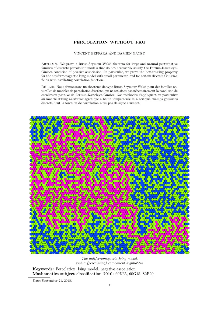
SLIDE 31

PERCOLATION WITHOUT FKG 31

define the random function fχ,L =

  • i∈N

aiχ(λi L )ϕi, where the ai are independent Gaussian random variables of variance 1, and (ϕi)i is a Hilbert

  • rthonormal basis of eigenfunctions of ∆ associated to the eigenvalues (λi)i. Then the asso-

ciated kernel Kχ,L, in normal coordinates near a point x0 = 0, satisfies (see [11]) ∀(x, y) ∈ Rn, KL( x L, y L) →

L→∞ Kχ(x, y),

where Kχ(x, y) =

  • ξ∈R2 χ(ξ2)ei<x−y,ξ>dξ.

The smoothness of χ implies that Kχ decays faster than any negative power of the distance. This model can be seen as an approximation of the random wave model, where χ = δ1. More precisely, consider the random sum of wave (A.1) ∀x ∈ R2, g(x) =

  • m=−∞

amJ|m|(r)eimϕ Here (r, ϕ) denotes the polar coordinates of x, Jk denotes the k-th Bessel function, and (am)m∈Z are independent normal coefficients. The correlation function for this model equals (see [6]) (A.2) K(x, y) =

  • ξ∈R2, ξ=1

ei<x−y,ξ>dξ = J0(x − y). In [5] and [6], the authors conjectured that the latter model should be related to some perco- lation model. Note that K decays polynomially in this distance with degree 1/2, so it does not enter our setting. The kernel Kχ defines a random Gaussian field fχ on R2, which we call here the smoothed random wave model associated to χ. Since J0 oscillates and since Kχ converges on compacts to K when χ → δ1, for every R > 0 and every degree d > 10, it gives an example of a correlation function satisfying the condition (1.1) with degree at least d, and which oscillates

  • utside the ball of radius R.

References

[1] V. Beffara and D. Gayet, Percolation of random nodal lines, to appear in Publ. Math. Inst. Hautes ´ Etudes Sci., arXiv:1605.08605, DOI: 10.1007/s10240-017-0093-0, (2016). [2] D. Beliaev and S. Muirhead, Discretisation schemes for level sets of planar Gaussian fields, arXiv preprint 1702.02134, (2017). [3] D. Beliaev, S. Muirhead, and I. Wigman, Russo-Seymour-Welsh estimates for the Kostlan ensemble

  • f random polynomials, arXiv preprint 1709.08961, (2017).

[4] J. van den Berg and C. Maes, Disagreement percolation in the study of Markov fields., Ann. Probab., 22 (1994), pp. 749–763. [5] E. Bogomolny and C. Schmit, Percolation model for nodal domains of chaotic wave functions, Phys.

  • Rev. Lett., 88 (2002), p. 114102.

[6] , Random wavefunctions and percolation, J. Phys. A, Math. Theor., 40 (2007), pp. 14033–14043. [7] H. Duminil-Copin, C. Hongler, and P. Nolin, Connection probabilities and RSW-type bounds for the two-dimensional FK Ising model, Communications on Pure and Applied Mathematics, 64 (2011),

  • pp. 1165–1198.

[8] G. Grimmett, Percolation, Berlin: Springer, 2nd ed. ed., 1999. [9] O. Haggstrom, J. Jonasson, and R. Lyons, Coupling and Bernoullicity in random-cluster and Potts models, Bernoulli, 8 (2001), pp. 275–294. [10] T. E. Harris, A lower bound for the critical probability in a certain percolation process, Mathematical Proceedings of the Cambridge Philosophical Society, 56 (1960), pp. 13–20. [11] L. H¨

  • rmander, The spectral function of an elliptic operator, Acta Math., 121 (1968), pp. 193–218.

[12] H. Kesten, Analyticity properties and power law estimates of functions in percolation theory, Journal of Statistical Physics, 25 (1981), pp. 717–756.

slide-32
SLIDE 32

32 VINCENT BEFFARA AND DAMIEN GAYET

[13] L. D. Pitt, Positively Correlated Normal Variables are Associated, The Annals of Probability, 10 (1982),

  • pp. 496–499.

[14] J. G. Propp and D. B. Wilson, Exact sampling with coupled Markov chains and applications to statistical mechanics, Random Structures and Algorithms, 9 (1996), pp. 223–252. [15] , Coupling from the past: A user’s guide., in Microsurveys in discrete probability. DIMACS work- shop, Princeton, NJ, USA, June 2–6, 1997, Providence, RI: AMS, American Mathematical Society, 1998,

  • pp. 181–192.

[16] A. Rivera and H. Vanneuville, Quasi-independence for nodal lines, arXiv preprint 1711.05009, (2017). [17] L. Russo, A note on percolation, Zeitschrift f¨ ur Wahrscheinlichkeitstheorie und Verwandte Gebiete, 43 (1978), pp. 39–48. [18] P. D. Seymour and D. J. A. Welsh, Percolation Probabilities on the Square Lattice, Annals of Discrete Mathematics, 3 (1978), pp. 227–245. [19] V. Tassion, Crossing probabilities for Voronoi percolation, Ann. Probab., 44 (2016), pp. 3385–3398.

  • Univ. Grenoble Alpes, CNRS, Institut Fourier, F–38000 Grenoble, France