FINAL EXAM REVIEW Will cover: All content from the course (Units - - PowerPoint PPT Presentation

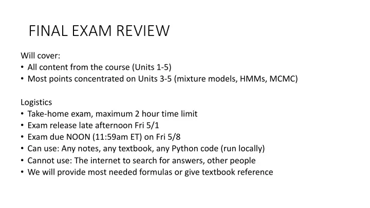
FINAL EXAM REVIEW

Will cover:

• All content from the course (Units 1-5)
• Most points concentrated on Units 3-5 (mixture models, HMMs, MCMC)

Logistics

• Take-home exam, maximum 2 hour time limit
• Exam release late afternoon Fri 5/1
• Exam due NOON (11:59am ET) on Fri 5/8
• Can use: Any notes, any textbook, any Python code (run locally)
• Cannot use: The internet to search for answers, other people
• We will provide most needed formulas or give textbook reference

Takeaway Messages

1) When uncertain about a variable, don’t condition on it, integrate it away! 2) Model performance is only as good as your fitting algorithm, initialization, and hyperparameter selection. 3) MCMC is a powerful way to estimate posterior distributions (and resulting expectations) even when the model is not analytically tractable

Takeaway 1!

When uncertain about a parameter, better to INTEGRATE AWAY than CONDITION ON OK: Using a point estimate BETTER: Integrate away ”w” via the sum rule

p(x∗| ˆ w)

p(x∗|X) = Z

w

p(x∗, w|X)dw

Takeaway 2

• Initialization, remember CP3 (GMMs)
• as well as CP5 (coming!)
• Algorithm, remember the difference between

LBFGS and EM in CP3 * Hyperparameter: Remember the poor performance in CP2

Difference between purple and blue is 0.01 on log scale When normalized over 400 pixels (20x20) per image Means purple model says average validation set image is exp(0.01 * 400) = 54.5 times more likely than the blue model

Takeaway 3

• Can use MCMC to do posterior predictive

p(x∗|X) = Z

w

p(x∗, w|X)dw = Z

w

p(x∗|w)p(w|X)dw = 1 S

S

X

s=1

p(x∗|ws), ws iid ∼ p(ws|X)

You are capable of so many things now!

Given a proposed probabilistic model, you can do:

ML estimation of parameters MAP estimation of parameters EM to estimate parameters MCMC estimation of posterior Heldout likelihood computation Hyperparameter selection via CV Hyperparameter selection via evidence

Unit 1

Probabilistic Analysis Skills

• Discrete and continuous r.v.
• Sum rule and product rule
• Bayes rule (derived from above)
• Expectations
• Independence

Distributions

• Bernoulli distribution
• Beta distribution
• Gamma function
• Dirichlet distribution

Data analysis

• Beta-Bernoulli for binary data
• ML estimation of ”proba. heads"
• MAP estimation of “proba. heads"
• Estimating the posterior
• Predicting new data
• Dirichlet-Categorical for discrete data
• ML estimation of unigram probas
• MAP estimation of unigram probas
• Estimating the posterior
• Predicting new data

Optimization Skills

• Finding extrema by zeros of first derivative
• Handling Constraints via Lagrange multipliers

Example Unit 1 Question

a) True or False: Bayes Rule can be proved using the Sum Rule and Product Rules a) You’re modeling the wins/losses of your favorite sports team with a Beta-Bernoulli model.

a) You assume each game’s binary outcome (win=1/loss=0) is iid. b) You observe in preseason play: 5 wins and 3 losses c) Suggest a prior to use for the win probability d) Identify 2 or more assumptions about this model that may not be valid in the real world (with concrete reasons)

Example Unit 1 Answer

Unit 2

Probabilistic Analysis Skills

• Joints, conditionals, marginals
• Covariance matrices (pos. definite, symmetric)
• Gaussian conjugacy rules

Linear Algebra Skills

• Determinants
• Positive definite
• Invertibility

Distributions

• Univariate Gaussian distribution
• Multivariate Gaussian distribution

Data analysis

• Gaussian-Gaussian for regression
• ML estimation of weights
• MAP estimation of weights
• Estimating the posterior over weights
• Predicting new data

Optimization Skills

• Convexity and second derivatives
• Finding extrema by zeros of first derivative
• First and second order gradient descent

Example Unit 2 Question

You are doing regression with the following model

• Normal prior on the weights
• Normal likelihood:
• a. Consider the following two estimators for t_*. What’s the difference?
• b. Suggest at least 2 ways to pick a value for the hyperparameter \sigma

p(tn|xn) = NormPDF(w ∗ xn, σ2)

ˆ t∗ = wMAP x∗ ˜ t∗ = Et∼p(t|x∗,X)[t]

Example Unit 2 Answer

Unit 3: K-Means and Mixture Models

Distributions

• Mixtures of Gaussians (GMMs)
• Mixtures in general
• Can use any likelihood (not just Gauss)

Numerical Methods logsumexp Data analysis

• K-means or GMM for a dataset
• How to pick K hyperparameter
• Why multiple inits matter

Optimization Skills

• K-means objective and algorithm
• Coordinate ascent / descent algorithms
• Optimization objectives with hidden vars
• Complete likelihood: p(x, z | \theta)
• Incomplete likelihood: p( x | \theta)
• Expectations of complete likelihood
• How to derive it
• Why it is important
• Expectation-Maximization algorithm
• Lower bound objective
• What E-step does
• What M-step does

Ex Exampl ple Uni nit 3 Que uestion

Consider two possible models for clustering 1-dim. data

• K-Means
• Gaussian mixtures

Name ways that the GMM is more flexible as a model:

• How is the GMM’s treatment of assignments more flexible?
• How is the GMM’s parameterization of a “cluster” more flexible?

Under what limit does the GMM likelihood reduce to the K-means objective?

Ex Exampl ple Uni nit 3 An Answer

Unit 4: Markov models and HMMs

Probabilistic Analysis Skills

• Markov conditional independence
• Stationary distributions
• Deriving independence properties
• Like HW4 problem 1

Linear Algebra Skills

• Eigenvectors/values for stationary

distributions Distributions

• Discrete Markov models

Algorithm Skills

• Forward algorithm
• Backward algorithm
• Viterbi algorithm

(all examples of dynamic programming) Optimization Skills

• EM for HMMs
• E-step
• M-step

Example Unit 4 Question

• Describe how the Viterbi algorithm is an instance of dynamic programming

Identify all the key parts:

• What is the fundamental problem being solved?
• How is the final solution built from solutions to smaller problems?
• How to describe all the solutions as a big “table” that should be filled in?
• What is the “base case” update (the simplest subproblem)?
• What is the recursive update?

Example Unit 4 Answer

Unit 5: Markov Chain Monte Carlo

Probabilistic Analysis Skills

• Inverse CDF rule for sampling
• Transformations of random variables
• Ancestral sampling
• Stationary distributions
• Remember, always a unique stationary

distribution if Markov chain is ergodic

• Detailed balance

Linear Algebra Skills

• Eigenvectors/values for stationary

distributions

MCMC algorithms

• Metropolis
• Metropolis-Hastings
• Gibbs sampling

Data Analysis

• Using MCMC to estimate a posterior

Example Unit 5 Question

• 5a. Can we use the inverse CDF rule for sampling from a univariate

Normal analytically? Can we do it numerically? If so, how?

• 5b. How would you use ancestral sampling to sample from a Bayesian

Linear regression model?

• 5c. T/F: We only need to run one MCMC chain in practice and we can

use all samples from that china

Example Unit 5 Answer