1 Baysian networks for decision analysis The TV show problem as a - - PDF document

1
SMART_READER_LITE
LIVE PREVIEW

1 Baysian networks for decision analysis The TV show problem as a - - PDF document

Several names Decision graphs Decision trees Influence diagrams Decision graphs I A certain kind of strictly symmetric decision trees Decisions and utilities No forgetting assumption LIMIDs Limited Memory


slide-1
SLIDE 1

1

Slide 1

Decision graphs I Decisions and utilities

Anders Ringgaard Kristensen

Slide 2

Several names

Decision graphs

  • Decision trees
  • Influence diagrams
  • A certain kind of strictly symmetric decision trees
  • “No forgetting” assumption
  • LIMIDs – Limited Memory Influence Diagrams
  • Influence diagrams without the “no forgetting”

assumption

Very often the terms “Decision graphs” and “Influence diagrams” are used synonymously.

Slide 3

Where are we?

First processing: Monitoring & filtering Second processing: Decision making Some methods integrate the whole setup

Bayesian Networks Decision Graphs

Slide 4

Bayesian networks to Decision graphs

If we have a Bayesian network and add:

  • Decision nodes
  • Utility nodes

Then we have a decision graph (if we obey certain rules) Algorithms for optimization of decisions are available

Slide 5

Notation, variables (= nodes)

C

Random variable, Chance node

D

Decision variable, Decision node D =

U

= U Utility variable, Utility node
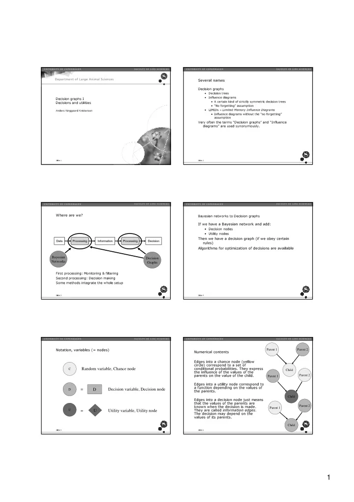
Slide 6

Numerical contents Edges into a chance node (yellow circle) correspond to a set of conditional probabilities. They express the influence of the values of the parents on the value of the child. Edges into a utility node correspond to a function depending on the values of the parents. Edges into a decision node just means that the values of the parents are known when the decision is made. They are called information edges. The decision may depend on the values of its parents.

Parent 1 Child Parent 2 Parent 1 Child Parent 2 Parent 1 Child Parent 2

slide-2
SLIDE 2

2

Slide 7

The TV show problem as a BN

Refer do demo file ShowBN.xbn

Opened True Choice 1 Choice 2 Gain

Slide 8

Baysian networks for decision analysis

Problems

  • More than one decision
  • Many combinations to test
  • The same decision is not necessarily the best

under all circumstances

  • Complex strategies
  • Cannot be entered as evidence
  • Need for direct optimization
Slide 9

Exercise

Use the notation on Slide 5 and the rules on Slide 6 to change the TV show problem on Slide 7 to a decision

  • graph. Consider:
  • Which nodes are actually decision nodes (from the

player’s point of view)?

  • Should we add any information edges?
Slide 10

Two kinds of decisions

Test decisions

  • The decision to
  • bserve the value of

a variable.

Actions

  • Influences the value
  • f at least one

variable.

  • In this case:
  • Fever
  • Tired
  • No influence on Flu

Flu Fever Tired

Test

Aspirin

Slide 11

Causal influences

The causal direction

Flu Fever Tired Flu Fever Tired

The reasoning direction

As long as we don’t include actions, the two Bayesian networks are equivalent If we include the action “Aspirin”, it would cure the flu in the latter case! In particular with decision graphs:

  • Be careful with

causality!

Slide 12

How to model a test decision

Include a “mirror variable” for the observed node:

  • The “mirror” has the same states AND a “not observed” state.

Flu Fever Tired Test Obs. fever

{No, yes} {Normal, medium, high} {No, yes} {No, yes} {Not observed, normal, medium, high}

slide-3
SLIDE 3

3

Slide 13

P(Obs. Fever | Fever, Test)

P(Obs. Fever | Fever, Test)

1 Medium 1 High Yes Medium 1 Yes Normal Normal Not observed Test Fever 1 No High 1 No Medium 1 No Normal Yes High

Slide 14

How to model the action

Include an “after-action” variable to capture the effect of the action.

  • The “after-action” variable typically has the same states as the original

variable.

Flu Fever Test Obs. fever

{No, yes} {Normal, medium, high} {No, yes} {No, yes} {Not observed, normal, medium, high}

Tired Fever’ Aspirin

{No, yes} {Normal, medium, high}

Slide 15

Does it pay to perform tests?

What is the benefit?

  • Costs of test.
  • Improvement in “result”

Will the result change your actions?

  • Are there any intervening options?
  • Can you trust the result of the test?
Slide 16

What is the benefit?

Fever example:

Flu Fever Test Obs. fever Tired Fever’ Aspirin

Benefit Cost: Inconvenience Cost: Price of aspirin

Inconv Price

Slide 17

What is the total benefit? Consequences:

  • Less tired
  • Inconvenience of fever test
  • Price of aspirin

Not comparable – cannot be added! We need a common unit for measurement The utility concept – a well known theory

Slide 18

Multi attribute utility: two attributes

Monetary gain “Well-being” Low Medium High )u )u 1 1 )u )u21 22
slide-4
SLIDE 4

4

Slide 19

Utility concept in decision graphs

Decision graphs don’t support varying marginal rates of substitution between attributes. The values of all utility nodes of the graph are just summed and maximized. All utilities must be expressed in the same unit (e.g. money). No time preference allowed.

Slide 20

Constant marginal rate of substitution

Monetary gain Well being Low Medium High )u )u )u )u 1 2 1 2 Slide 21

Will the result change your actions?

The fever example:

  • The aspirin action is the obvious and natural consequence of

the test.

  • But, what about just taking an aspirin (without testing)?
  • Inconvenience of test
  • Cost of aspirin
  • “You are not allowed to do that” – if true, a utility node

is missing!

  • Reliability of test
Slide 22

Will the result change your actions?

The simple milk test example (example from Tuesday):

  • The obvious action is not to pour the milk from a positive

test into the bulk tank.

  • We would never do that unless we think the milk is infected.
  • But, what about just pouring the milk into the bulk tank

(without testing)?

  • Cost of test
  • Loss from delivering infected milk to the dairy
  • Reliability of test
Slide 23

Reliability of milk test 0.99 0.01

Infected = ”no”

0.01 0.99

Infected = ”yes” Test = negative Test = positive

Infected Test

0.9993 0.0007

Infected = ”no” Infected = ”yes”

What is the probability that a positive test is right?

Slide 24

Reliability of diagnostic tests

What is the probability that a Danish cow is suffering from “mad cow disease”? What are the sensitivity and specificity of the test for “mad cow disease”? Reasoning against the causal direction. Conclusion?

slide-5
SLIDE 5

5

Slide 25

In some situations it matters

Morgenthaler in Politiken:
  • Honey, did you know that the prior likelihood of an event like this is extremely small?
Slide 26

The cow feeding example

Should we perform laboratory analyses of roughages fed to dairy cows? Depends on:

  • The precision of the analysis
  • The herd size
  • The cost of the analyses
  • The relative amount of roughages fed
  • The uncertainty of the milk yield response to the nutritional

contents

For simplicity:

  • Only energy content considered
  • Only one roughage and one concentrate
Slide 27

The cow feeding example

The obvious action as a consequence of the test result is to adjust the proportion of roughages relative to concentrates in the ration.

Slide 28

The cow feeding examble

Test Action

Slide 29

Decision trees

A very common technique for evaluation of alternative decisions over time. In particular popular in the veterinary community. Example diseased calf:

  • Treat: Yes/no
  • Cost of treatment: 100 DKK
  • Value of surviving calve: 1650 DKK
  • Survival of animals:
  • Treated: 0.88
  • Untreated: 0.60
Slide 30

Decision tree for diseased calf

Value of decision “Yes”:

  • 0.88 × 1650 + 0.12 × (-70) – 100 = 1343.60

Value of decision “No”:

  • 0.60 × 1650 + 0.40 × (-70) = 962

The optimal decision is obviously to treat.

Treat Die Die

Y: -100 N: 0 N: 0.88 Y: 0.12

  • 70

1650

  • 70

1650

Untreated, dead Untreated, survived Treated, dead Treated, survived

N: 0.60 Y: 0.40

slide-6
SLIDE 6

6

Slide 31

The treatment problem as a decision graph

Refer to file “Treatment.xbn” The answers are (fortunately) the same as with the decision tree. Any decision graph can be modeled as a decision tree.

Slide 32

A tiny part of the cow feeding problem

Number of leaves: 3 × 4 × 5 × 5 = 300 (only 5 shown) That’s why we need decision graphs! Hidden assumptions (e.g. true value for silage).

Me HS Me Me Obs Obs

Obs

Obs Mix Mix Mix R R

R

R R Mix Mix