1 Lecture Overview Nonlinearity and Gamma Many basic things tying - - PDF document

▶

Aug 15, 2023 331 likes •390 views

Lecture Overview Foundations of Computer Graphics Many basic things tying together course Is part of the material, will be covered on midterm (Fall 2012) Raster graphics CS 184, Lecture 12: Raster Graphics and Pipeline

SLIDE 1

1 Foundations of Computer Graphics (Fall 2012)

CS 184, Lecture 12: Raster Graphics and Pipeline

http://inst.eecs.berkeley.edu/~cs184

Lecture Overview

§ Many basic things tying together course

§ Is part of the material, will be covered on midterm

§ Raster graphics § Gamma Correction § Color § Hardware pipeline and rasterization § Displaying Images: Ray Tracing and Rasterization

§ Essentially what this course is about (HW 2 and HW 5)

§ Introduced now so could cover basics for HW 1,2,3

§ Course will now “breathe” to review some topics Some images from wikipedia

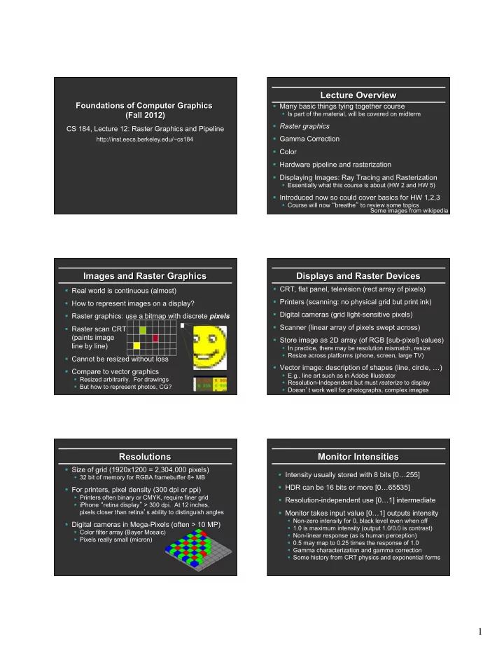
Images and Raster Graphics

§ Real world is continuous (almost) § How to represent images on a display? § Raster graphics: use a bitmap with discrete pixels § Raster scan CRT (paints image line by line) § Cannot be resized without loss § Compare to vector graphics

§ Resized arbitrarily. For drawings § But how to represent photos, CG?

Displays and Raster Devices

§ CRT, flat panel, television (rect array of pixels) § Printers (scanning: no physical grid but print ink) § Digital cameras (grid light-sensitive pixels) § Scanner (linear array of pixels swept across) § Store image as 2D array (of RGB [sub-pixel] values)

§ In practice, there may be resolution mismatch, resize § Resize across platforms (phone, screen, large TV)

§ Vector image: description of shapes (line, circle, …)

§ E.g., line art such as in Adobe Illustrator § Resolution-Independent but must rasterize to display § Doesn’t work well for photographs, complex images

Resolutions

§ Size of grid (1920x1200 = 2,304,000 pixels)

§ 32 bit of memory for RGBA framebuffer 8+ MB

§ For printers, pixel density (300 dpi or ppi)

§ Printers often binary or CMYK, require finer grid § iPhone “retina display” > 300 dpi. At 12 inches, pixels closer than retina’s ability to distinguish angles

§ Digital cameras in Mega-Pixels (often > 10 MP)

§ Color filter array (Bayer Mosaic) § Pixels really small (micron)

Monitor Intensities

§ Intensity usually stored with 8 bits [0…255] § HDR can be 16 bits or more [0…65535] § Resolution-independent use [0…1] intermediate § Monitor takes input value [0…1] outputs intensity

§ Non-zero intensity for 0, black level even when off § 1.0 is maximum intensity (output 1.0/0.0 is contrast) § Non-linear response (as is human perception) § 0.5 may map to 0.25 times the response of 1.0 § Gamma characterization and gamma correction § Some history from CRT physics and exponential forms

SLIDE 2

2 Lecture Overview

§ Many basic things tying together course § Raster graphics § Gamma Correction § Color § Hardware pipeline and rasterization § Displaying Images: Ray Tracing and Rasterization

§ Essentially what this course is about (HW 2 and HW 5) Some images from wikipedia

Nonlinearity and Gamma

§ Exponential function § I is displayed intensity, a is pixel value § For many monitors γ is between 1.8 and 2.2 § In computer graphics, most images are linear

§ Lighting and material interact linearly

§ Gamma correction § Examples with γ = 2

§ Input a = 0 leads to final intensity I = 0, no correction § Input a = 1 leads to final intensity I = 1, no correction § Input a = 0.5 final intensity 0.25. Correct to 0.707107 § Makes image “brighter” [brightens mid-tones]

I = aγ a' = a

1 γ

Gamma Correction

§ Can be messy for images. Usually gamma

n one monitor, but viewed on others…

§ For television, encode with gamma (often 0.45, decode with gamma 2.2) § CG, encode gamma is usually 1, correct

www.dfstudios.co.uk/wp-content/ uploads/2010/12/graph_gamcor.png

Finding Monitor Gamma

§ Adjust grey until match 0-1 checkerboard to find mid-point a value i.e., a for I = 0.5

I = aγ γ = log0.5 loga

Human Perception

§ Why not just make everything linear, avoid gamma § Ideally, 256 intensity values look linear § But human perception itself non-linear

§ Gamma between 1.5 and 3 depending on conditions § Gamma is (sometimes) a feature § Equally spaced input values are perceived roughly equal

Lecture Overview

§ Many basic things tying together course § Raster graphics § Gamma Correction § Color § Hardware pipeline and rasterization § Displaying Images: Ray Tracing and Rasterization

§ Essentially what this course is about (HW 2 and HW 5) Some images from wikipedia

SLIDE 3

3 Color

§ Huge topic (can read textbooks)

§ Schrodinger much more work on this than quantum

§ For this course, RGB (red green blue), 3 primaries § Additive (not subtractive) mixing for arbitrary colors § Grayscale: 0.3 R + 0.6 G + 0.1 B § Secondary Colors (additive, not paints etc.)

§ Red + Green = Yellow, Red + Blue = Magenta, Blue + Green = Cyan, R+G+B = White

§ Many other color spaces

§ HSV, CIE etc.

RGB Color

§ Venn, color cube § Not all colors possible

Images from wikipedia

Eyes as Sensors

Slides courtesy Prof. O’Brien

Cones (Trichromatic) Cone Response Color Matching Functions

SLIDE 4

4 CIE XYZ Alpha Compositing

§ RGBA (32 bits including alpha transparency)

§ You mostly use 1 (opaque) § Can simulate sub-pixel coverage and effects

§ Compositing algebra

Lecture Overview

§ Many basic things tying together course § Raster graphics § Gamma Correction § Color § Hardware pipeline and rasterization § Displaying Images: Ray Tracing and Rasterization

§ Essentially what this course is about (HW 2 and HW 5) Read chapter 8 more details

Hardware Pipeline

§ Application generates stream of vertices § Vertex shader called for each vertex

§ Output is transformed geometry

§ OpenGL rasterizes transformed vertices

§ Output are fragments

§ Fragment shader for each fragment

§ Output is Framebuffer image

Rasterization

§ In modern OpenGL, really only OpenGL function

§ Almost everything is user-specified, programmable § Basically, how to draw (2D) primitive on screen

§ Long history

§ Bresenham line drawing § Polygon clipping § Antialiasing

§ What we care about

§ OpenGL generates a fragment for each pixel in triangle § Colors, values interpolated from vertices (Gouraud)

Z-Buffer

§ Sort fragments by depth (only draw closest one) § New fragment replaces

ld if depth test works

§ OpenGL does this auto can override if you want § Must store z memory § Simple, easy to use

SLIDE 5

5 Lecture Overview

§ Many basic things tying together course § Raster graphics § Gamma Correction § Color § Hardware pipeline and rasterization § Displaying Images: Ray Tracing and Rasterization

§ Essentially what this course is about (HW 2 and HW 5)

What is the core of 3D pipeline?

§ For each object (triangle), for each pixel, compute shading (do fragment program) § Rasterization (OpenGL) in HW 2

§ For each object (triangle)

§ For each pixel spanned by that triangle

§ Call fragment program

§ Ray Tracing in HW 5: flip loops

§ For each pixel

§ For each triangle

§ Compute shading (rough equivalent of fragment program)

§ HW 2, 5 take almost same input. Core of class

Ray Tracing vs Rasterization

§ Rasterization complexity is N * d

§ (N = objs, p = pix, d = pix/object) § Must touch each object (but culling possible)

§ Ray tracing naïve complexity is p * N

§ Much higher since p >> d § But acceleration structures allow p * log (N) § Must touch each pixel § Ray tracing can win if geometry very complex

§ Historically, OpenGL real-time, ray tracing slow

§ Now, real-time ray tracers, OpenRT, NVIDIA Optix § Ray tracing has advantage for shadows, interreflections § Hybrid solutions now common

Course Goals and Overview

§ Generate images from 3D graphics § Using both rasterization (OpenGL) and Raytracing