1 Data structures for decoder: Construction of canonical Huffman: - - PDF document

SLIDE 1

1

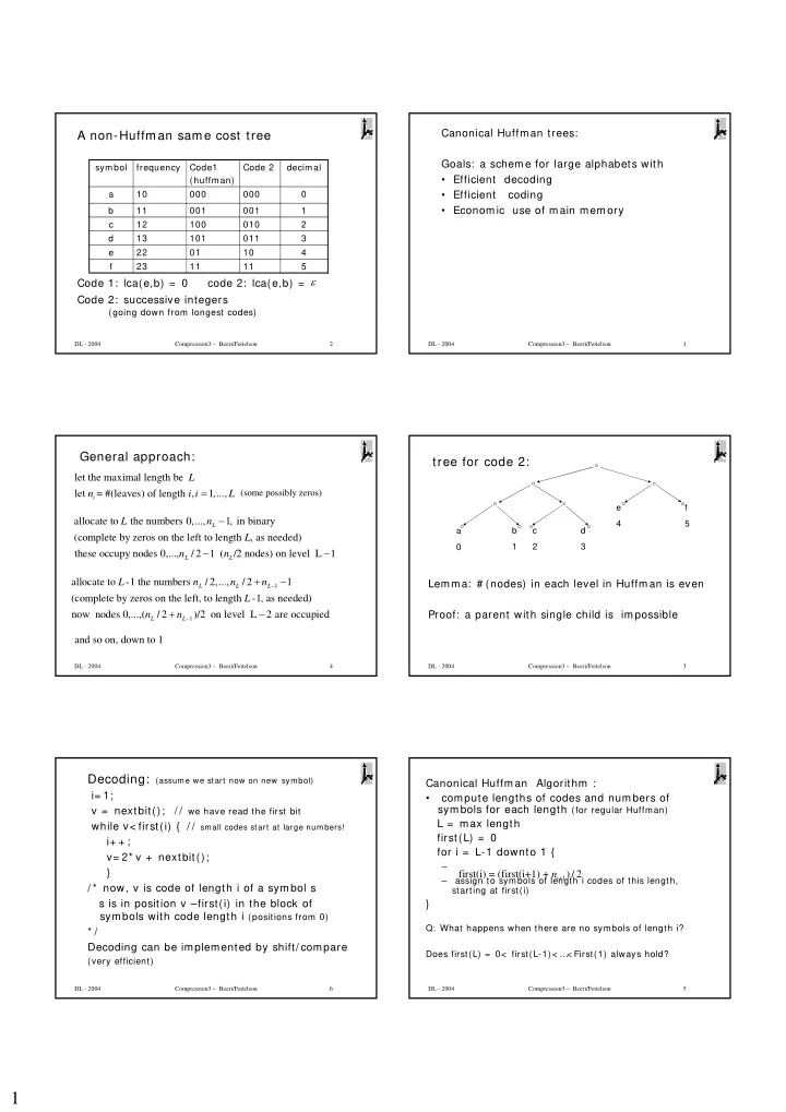
DL - 2004 Compression3 – Beeri/Feitelson 1

Canonical Huffman trees: Goals: a scheme for large alphabets with

• Efficient decoding
• Efficient coding
• Economic use of main memory

DL - 2004 Compression3 – Beeri/Feitelson 2

A non-Huffman same cost tree

Code 1: lca(e,b) = 0 code 2: lca(e,b) = Code 2: successive integers

(going down from longest codes) 5 4 3 2 1 decimal 11 11 23 f Code 2 Code1 (huffman) frequency symbol 10 01 22 e 011 101 13 d 010 100 12 c 001 001 11 b 000 000 10 a

ε

DL - 2004 Compression3 – Beeri/Feitelson 3

tree for code 2:

Lemma: # (nodes) in each level in Huffman is even Proof: a parent with single child is impossible

a b 1 c 2 d 3 e 4 f 5

DL - 2004 Compression3 – Beeri/Feitelson 4

General approach:

(some possibly zeros)

let the maximal length be let = #(leaves) of length , 1,...,

i

L n i i L = allocate to the numbers 0,..., 1, in binary (complete by zeros on the left to length , as needed) these occupy nodes 0,..., / 2 1 ( /2 nodes) on level L 1

L L L

L n L n n − − −

1 1

allocate to -1 the numbers / 2,..., / 2 1 (complete by zeros on the left, to length -1, as needed) now nodes 0,...,( / 2 )/2 on level L 2 are occupied

L L L L L

L n n n L n n

− −

+ − + − and so on, down to 1

DL - 2004 Compression3 – Beeri/Feitelson 5

Canonical Huffman Algorithm :

• compute lengths of codes and numbers of

symbols for each length (for regular Huffman) L = max length first(L) = 0 for i = L-1 downto 1 {

– – assign to symbols of length i codes of this length, starting at first(i)

}

Q: What happens when there are no symbols of length i? Does first(L) = 0< first(L-1)< … < First(1) always hold?

1

first(i) = (first(i+1) + ) / 2

i

n +

DL - 2004 Compression3 – Beeri/Feitelson 6

Decoding: (assume we start now on new symbol)

i= 1; v = nextbit(); / / we have read the first bit while v< first(i) { / / small codes start at large numbers! i+ + ; v= 2* v + nextbit(); } / * now, v is code of length i of a symbol s s is in position v –first(i) in the block of symbols with code length i (positions from 0) * / Decoding can be implemented by shift/ compare

(very efficient)

SLIDE 2

2

DL - 2004 Compression3 – Beeri/Feitelson 7

Data structures for decoder:

• The array first(i)
• Arrays S(i) of the symbols with code length i,
• rdered by their code

(v-first(i) is the index value to get the symbol for code v)

Thus, decoding uses efficient arithmetic operations + array look-up – more efficient then storing a tree and traversing pointers What about coding (for large alphabets, where symbols = words or blocks)? The problem: millions of symbols large Huffman tree, …

DL - 2004 Compression3 – Beeri/Feitelson 8

Construction of canonical Huffman: (sketch)

assumption: we have the symbol frequencies Input: a sequence of (symbol, freq) Output: a sequence of (symbol, length) Idea: use an array to represent a heap for creating the tree, and the resulting tree and lengths We illustrate by example

DL - 2004 Compression3 – Beeri/Feitelson 9

Example: frequencies: 2, 8, 11, 12

(each cell with a freq. also contains a symbol – not shown)

Now reps of 2, 8 (smallest) go out, rest percolate The sum 10 is put into cell4, and its rep into cell 3 Cell4 is the parent (“sum”) of cells 5, 8.

8 11 12 2 # 6 # 7 # 8 # 5 8 11 12 2 # 6 # 7 # 4 11 12 # 4 10 # 3 # 6 # 7

DL - 2004 Compression3 – Beeri/Feitelson 10

after one more step: Finally, a representation of the Huffman tree: Next, by i= 2 to 8, assign lengths (here shown after i= 4)

# 4 # 3 12 # 4 # 3 21 # 3 # 6 # 4 # 3 # 2 # 4 # 3 # 2 33 # 2 # 4 # 3 # 2 # 4 2 1 # 2

DL - 2004 Compression3 – Beeri/Feitelson 11

Summary:

• Insertion of (symbol,freq) into array – O(n)
• Creation of heap –
• Creating tree from heap: each step is

total is

• Computing lengths O(n)
• Storage requirements: 2n (compare to tree!)

log kn n log k n log kn n

DL - 2004 Compression3 – Beeri/Feitelson 12

Entropy H: a lower bound on compression How can one still improve?

Huffman works for given frequencies, e.g., for the English language – static modeling Plus: No need to store model in coder/ decoder But, can construct frequency table for each file semi-static modeling Minus:

– Need to store model in compressed file (negligible for large files) – Takes more time to compress

Plus: may provide for better compression

SLIDE 3

3

DL - 2004 Compression3 – Beeri/Feitelson 13

3rd option: start compressing with default freqs As coding proceeds, update frequencies: After reading a symbol:

– compress it – update freq table*

Adaptive modeling Decoding must use precisely same algorithm for updating freqs can follow coding Plus:

• Model need not be stored
• May provide compression that adapts to file,

including local changes of freqs Minus: less efficient then previous models * May use a sliding window to better reflect local changes

DL - 2004 Compression3 – Beeri/Feitelson 14

Adaptive Huffman:

• Construction of Huffman after each symbol: O(n)
• Incremental adaptation in O(logn) is possible

Both too expensive for practical use (large alphabets) We illustrate adaptive by arithmetic coding (soon)

DL - 2004 Compression3 – Beeri/Feitelson 15

Higher-order modeling: use of context e.g.: for each block of 2 letters, construct freq. table for the next letter (2-order compression)

(uses conditional probabilities – hence improvement)

This also can be static/ semi-static/ adaptive

DL - 2004 Compression3 – Beeri/Feitelson 16

Arithmetic coding:

Can be static, semi-static, adaptive Basic idea:

• Coder: start with the interval [ 0,1)
• 1st symbol selects a sub-interval, based on its

probability

• i’th symbol selects a sub-interval of (i-1)’th

interval, based on its probability

• When file ends, store a number in the final

interval

• Decoder: reads the number, reconstructs the

sequence of intervals, i.e. symbols

• Important: Length of file stored at beginning
• f compressed file

(otherwise, decoder does not know when to stop)

DL - 2004 Compression3 – Beeri/Feitelson 17

Example: (static) a ~ 3/ 4, b ~ 1/ 4

The file to be compressed: aaaba The sequence of intervals (& symbols creating them): [ 0,1), a [ 0,3/ 4), a [ 0,9/ 16), a [ 0, 27/ 64), b [ 81/ 256, 108/ 256), a [ 324/ 1024, 405/ 1024) Assuming this is the end, we store:

• 5 –length of file
• Any number in final interval, say 0.011 (3 digits)

(after first 3 a’s, one digit suffices!) (for a large file, the length will be negligible)

DL - 2004 Compression3 – Beeri/Feitelson 18

Why is it a good approach in general? For a symbol with large probability, # of binary digits needed to represent an occurrence is smaller than 1 poor compression with Huffman But, arithmetic represents such a symbol with a small shrinkage of interval, hence the extra number of digits is smaller than 1! Consider the example above, after aaa

SLIDE 4

4

DL - 2004 Compression3 – Beeri/Feitelson 19

Arithmetic coding – adaptive – an example: The symbols: { a, b, c} Initial frequencies: 1,1,1 (= initial accumulated freqs)

(0 is illegal, cannot code a symbol with probability 0!)

b: model passes to coder the triple (1, 2, 3):

– 1 : the accumulated freqs up to, not including, b – 2 : the accumulated freqs up to, including, b – 3 : the sum of freqs

Coder notes new interval [ 1/ 3, 2/ 3) Model updates freqs to 1, 2, 1 c: model passes (3,4,4) (upper quarter) Coder updates interval to [ 7/ 12,8/ 12) Model updates freqs to (1,2,2)

And so on … .

DL - 2004 Compression3 – Beeri/Feitelson 20

Practical considerations:

• Interval ends are held as binary numbers
• # of bits in number to be stored proportional

to size of file – impractical to compute it all before storing solution: as interval gets small, first bit of a number in it is determined. This bit is written by code into compressed file, and “removed” from interval ends (= mult by 2) Example: in 1st example, when interval becomes [ 0,27/ 64] ~ [ 000000,011011) (after 3 a’s)

• utput 0, and update to [ 00000,11011)

Decoder sees 1st 0: knows the first three are a’s, Computes interval, “throws” the 0

DL - 2004 Compression3 – Beeri/Feitelson 21

• Practically, (de)coder maintain a word for each

number, computations are approximate Some (very small) loss of compression Both sides must perform same approximations at “same time”

• Initial assignment of freq. 1 to

low freq. symbols? Solution: assign 1 to all symbols not seen so far If k were not seen yet, one now occurs, give it 1/ k

• Since coder does not know when to stop, file

length must be stored in compressed file

DL - 2004 Compression3 – Beeri/Feitelson 22

• Frequencies data structure: need to allow both

update, and sums of the form

(expensive for large alphabets)

Solution: a tree-like structure O(logn) accesses!

f1+ … + f8 1000 8 f7 111 7 f5+ f6 110 6 f5 101 5 f1+ f2+ f3+ f4 100 4 f3 11 3 f1+ f2 10 2 f1 1 1 sum binary cell

If k, the binary cell # ends with i 0’s, the cell contains fk+ f_(k-1)+ … + f_(k-i+ 1) What is the algorithm to compute

i i k

f

≤

∑

i i k

f

≤

∑

DL - 2004 Compression3 – Beeri/Feitelson 23

Dictionary-based methods

Huffman is a dictionary-based method: Each symbol in dictionary has associated code But, adaptive Huffman is not practical Famous adaptive methods: LZ77, LZ78 (Lempel-Ziv) We describe LZ77 (basis of gzip in Unix)

DL - 2004 Compression3 – Beeri/Feitelson 24

Basic idea: The dictionary -- the sequences of symbols in a window before current position (typical window size: )

• When coder at position p, window is the

symbols in positions p-w,… p-1

• Coder searches for longest seq. that matches

the one at position p

• If found, of length l, put (n,l) into file (n --
• ffset, l length), and forward l positions,

else output the current symbol

12 14

2 2 −

SLIDE 5

5

DL - 2004 Compression3 – Beeri/Feitelson 25

Example:

• input is: a b a a b a b…

b (11 b’s)

• Code is : a b (2,1) (1,1) (3,2) (2,1) (1,10)
• Decoding: a a, b b, (2,1) a, (1,1) a,

current known string: a b a a (3,2) b a, (2,1) b current known string: a b a a b a b (1, 10) Go back one step to b do 10 times: output scanned symbol, advance one

(note: run-length encoding hides here)

Note: decoding is extremely fast!

DL - 2004 Compression3 – Beeri/Feitelson 26

Practical issues: 1) Maintenance of window: use cyclic buffer 2) searching for longest matching word expensive coding 3) How to distinguish a pair (n,l) from a symbol? 4) Can we save on the space for (n,l)? The gzip solution for 2-4: 2: a hash table of 3-sequences, with lists of positions where a sequence starting with them exists (what about short matches?) An option: limit the search in the list (save time)

Does not always find the longest match, but loss is very small

DL - 2004 Compression3 – Beeri/Feitelson 27

3: one bit suffices (but see below) 4: offsets are integers in range [ 1,2^ k] , often smaller values are more frequent Semi-static solution: (gzip)

• Divide file into segments of 64k; for each:
• Find the offsets used and their frequencies
• Code using canonical Huffman
• Do same for lengths
• Actually, add symbols (issue 3) to set of

lengths, code together using one code, and put in file this code before offset code (why?)

DL - 2004 Compression3 – Beeri/Feitelson 28

One last issue (for all methods): synchronization Assume you want to start decoding in mid-file? E.g.: a db of files, coded using one code

• Bit-based addresses for the files --- these

addresses occur in many IL’s, which are loaded to MM. 32/ address is ok, 64/ address may be costly

• Byte/ word-based addresses allow for much

larger db’s. It may pay to even use k-word blocks based addresses how does one synchronize?

DL - 2004 Compression3 – Beeri/Feitelson 29

Solution: fill last block with 01… 1 if code fills last block, add a block Since file addresses/ lengths are known, filling can be removed Does this work for Huffman? Arithmetic? LZ77? What is the cost?

DL - 2004 Compression3 – Beeri/Feitelson 30

Summary of file compression:

• Large db’s compression helps reduce storage
• Fast query processing requires synchronization

and fast decoding

• Db is often given, so statistics can be collected –

semi-static is a viable option (plus regular re-organization)

• Context-based methods give good compression,

but expensive decoding word-based Huffman is recommended (semi-static)

• Construct two models: one for words, another

for no-words

SLIDE 6

6

DL - 2004 Compression3 – Beeri/Feitelson 31

Compression of inverted lists

Introduction Global, non-parametric methods Global parametric methods Local parametric methods

DL - 2004 Compression3 – Beeri/Feitelson 32

Introduction:

Important parameters:

• N - # of documents in db
• n - # of (distinct) words
• F - # of word occurrences
• f - # of inverted list entries

The index contains: lexicon (MM, if possible), IL’s (Disc) IL compression helps to reduce size of index, cost of i/ o (in TREC, 99) 741,856 535,346 333,338,738 134,994,414 Total size: 2G

DL - 2004 Compression3 – Beeri/Feitelson 33

The IL for a term t contains entries An entry: d (= doc. id), { in-doc freq. , in-doc-position,… } For ranked answers, the entry is usually (d, ) We consider each separately – independent compressions, can be composed

d,t

f

d,t

f

t

f

DL - 2004 Compression3 – Beeri/Feitelson 34

Compression of doc numbers: A sequence of numbers in [ 1..N] ; how can it be compressed? Most methods use gaps : g1= d1, g2= d2-d1, … We know that

• For long lists, most are small.

These facts can be used for compression

(Each method has an associated probability distribution

• n the gaps, defined by code lengths: )

i

g N ≤

∑

log(1/ )

i i

l p ∼

DL - 2004 Compression3 – Beeri/Feitelson 35

Global, non-parametric methods

Binary coding: represent each gap by a fixed length binary number Code length for g: Probability: uniform distribution: p(g)= 1/ N log N

DL - 2004 Compression3 – Beeri/Feitelson 36

Unary coding: represent each g> 0 by d-1 digits 1, then 0 1 -> 0, 2 -> 10, 3 -> 110, 4-> 1110, … Code length for g: g

• Worst case for sum: N (hence for all IL’s: nN)

is this a nice bound? P(g): Exponential decay; if does not hold in practice compression penalty

t

i f

g d =

∑

2 g

−

SLIDE 7

7

DL - 2004 Compression3 – Beeri/Feitelson 37

Gamma ( ) code : a number g is represented by

• Prefix אשיר: unary code for*
• Suffix אפיס: binary code, with digits,

for Examples:

(* Why not ?)

γ 1 log g +     log g    

log

2

g

d

   

− 1: 1 log1 1, prefix is 0, suffix is empty, code is 0 + =     7 : 1 log7 3, prefix is 110, suffix is 11, code is 11011 + =     18: Code length for g: 1 2 log g +    

(1 2 log ) 2 2

1 1 Probability: ( ) 2 2 2

g

p g g g

− + −    

= ≈ =

log g

   

DL - 2004 Compression3 – Beeri/Feitelson 38

Delta ( ) code : δ

log

prefix: represent 1 log in gamma code suffix: represent 2 in binary (as in gamma)

g

g g

   

+     − 7: 1 log7 3, 1 log3 2, prefix is 101 suffix is 11, code is 10111 0: : + = + =         Examples

(1 2 1 log log ) 2

Code lenght for g: 1 2 log(1 log ) log 1 2loglog log 1 Probability: ( ) 2 2 (log )

g g

g g g g p g g g

− + + +            

+ + +             + + = ≈

• DL - 2004

Compression3 – Beeri/Feitelson 39

Interim summary: We have codes with probability distributions : Q: can you prove that the (exact) formulas for probabilities for gamma, delta sum to 1?

2 2

unary gamma delta binary 1 1 2 log 2 2 (log )

g

N g g g

− DL - 2004 Compression3 – Beeri/Feitelson 40

Golomb code: Semi-static, uses db statistics global, parametric code 1) Select a basis b (based on db statistics – later) 2) g> 0 we represent g-1

• Prefix: let (integer division)

represent, in unary, q+ 1

• Suffix: the remainder is (g-1)-qb (in [ 0..b-1] )

represent by a binary tree code

• some leaves at distance
• the others at distance

( 1) / q g b = −     logb     logb    

DL - 2004 Compression3 – Beeri/Feitelson 41

The binary tree code: cut 2j leaves from the full binary tree of depth k assign leaves, in order, to the values in [ 0..b-1] Example: b= 6 let log , 2k k b j b = = −    

1 2 3 4 5

DL - 2004 Compression3 – Beeri/Feitelson 42

Summary of Golomb code: Exponential decay like unary, slower rate, affected by b Q: what is the underlying theory? Q: how is b chosen? Prefix: unary code of 1 ( 1) / Suffix: code of length between log and log g b b b + −            

( 1)/ 1/ 1

length 1 ( 1) / log 1 1 1 1 probability 2 2 2 (2 )

g b b g

g b b b b

− −

≈ + − +         ≈ ⋅ ≈ ⋅

SLIDE 8

8

DL - 2004 Compression3 – Beeri/Feitelson 43

Infinite Huffman Trees :

Example: Consider The code (* ) 0, 10, 110, 1110, … seems natural, but Huffman algorithm is not applicable! (why?) For each m, consider the (finite) m-approximation

• each has a Huffman tree code: 0, 10, …

, 1… 10

• the code for m+ 1 refines that of m
• The sequence of codes converges to (* )

( ) 2 , 1,....

i

p i i

−

= = 1 1 1 1 1 1 , ,..., , , where the last entry is 2 4 2 2 2 2

m m m i i m >

= ∑

DL - 2004 Compression3 – Beeri/Feitelson 44

1 1 1 1/2 1/4 1/4 1/8 1/8 1/2 approximation 1, code words: 0, 1 approximation 2, code words: 0, 10,11 1 approximation 3, code words: 0, 10,110,111 approximation 1, code words: 0, 10, 110, 1110, 1111 1/16 1/16

DL - 2004 Compression3 – Beeri/Feitelson 45

A more general approximation scheme: Given: the sequence An m-approximation, with skip b is the finite sequence where for example: b = 3:

1 2

, ,........ a a

1,..., m i m i jb i b j

a a

+ + + = ≥

= ∑

• 1

2 1

, ,..., , ,...,

m m m b

a a a a a

+ +

• 7

a

• 8

a

• 9

a

• approximated tail

DL - 2004 Compression3 – Beeri/Feitelson 46

Fact: refining the m-approx. by splitting to and gives the m+ 1-approx. A sequence of m-approximations is good if (* ) are the smallest in the sequence, so they are the 1st pair merged by Huffman

(why is this important?)

(* ) Depends on the and on b

1 m

a

+

• 1

m

a

+ 1 m b

a

+ +

• 1

1

,

m m b

a a

+ + +

• 1

2 1 2 1

, ,..., , , ..., ,

m m m m b m b

a a a a a a a

+ + + + +

• i

a

DL - 2004 Compression3 – Beeri/Feitelson 47

Let -- the Bernoulli distribution A decreasing sequence

• to prove (* ), need to show:

For which b do they hold?

1

(1 )i

i

a p p

−

= − ⋅

1 2

........ a a > >

1 1 1

is smallest among ,...,

m m

a a a

+ + 1 2 1

is smallest among ,...,

m b m m b

a a a

+ + + + +

• 1

a

1 m

a

+ 1 m b

a

+ +

• 2

m

a

+

• 1

(ii)

m b m

a a

+ + ≤

• 1

(i)

m m b

a a

+ +

≤

DL - 2004 Compression3 – Beeri/Feitelson 48

1

1 1

(1 ) (1 ) (1 ) 1 (1 ) 1 (1 )

m i jb

m i jb m i m i jb j j j m i b

a a p p p p p p p p

+ + −

+ − + + + ≥ ≥ ≥ + −

= = − ⋅ = − ⋅ ⋅ − = − ⋅ ⋅ − −

∑ ∑ ∑

• 1 1

1 1

1 Hence, (i) (1 ) (1 ) 1 (1 ) 1 (1 ) (1 )

m m b b b b

p p p p p p p

+ − + − −

⇒ − ⋅ ≤ − ⋅ ⋅ − − ⇒ ≤ − + −

1 1 1 1

1 And, (ii) (1 ) (1 ) 1 (1 ) (1 ) (1 ) 1

m b m b b b

p p p p p p p

+ − + − +

⇒ − ⋅ ⋅ ≤ − ⋅ − − ⇒ − + − ≤

1 1

(1 ) (1 ) 1 (1 ) together (1 )

b b b b

p p p p

+ −

− + − ≤ ≤ − + −

SLIDE 9

9

DL - 2004 Compression3 – Beeri/Feitelson 49

We select < on the right (useful later): has a unique solution To solve, from the left side, we obtain Hence the solution is (b is an integer):

1 1

(1 ) (1 ) 1 (1 ) (1 (**) )

b b b b

p p p p

+ −

− + − ≤ < − + − 1 (1 ) [1 1] 1 (1 ) 2 log(2 ) log(1 ) log(2 ) log(1 )

b b

p p p p p b p p b p − − + ≤ ⇒ − ≤ − − ⇒ ⋅ − ≤ − − ⇒ ≥ − − log(2 log(1 ) p b p   − = −   −  

DL - 2004 Compression3 – Beeri/Feitelson 50

Next: how do these Huffman trees look like? Start with 0-approx. Facts:

• 1. A decreasing sequence (so last two are smallest)

2.

(when b> 3)

follows from and (* * )

• 3. Previous two properties are preserved when

last two are replaced by their sum

• 4. The Huffman tree for the sequence assigns to

codes of lengths of same cost as the Golomb code for remainders Proof: induction on b

1,..., b

a a

• 1

1 b b

a a a

− +

>

• 1

1 (1 ) 1 (1 )

i i b

a p p p

−

= ⋅ − ⋅ − −

• log
• r log

b b        

DL - 2004 Compression3 – Beeri/Feitelson 51

Now, expand the approximations, to obtain infinite tree: This is the Golomb code, (with places of prefix/ suffix exchanged)!! To obtain code for start from and split times

qb j j

a a q

+

• 1

1 1

j

a

• j b

a +

• j

a

2 j b

a +

• j b

a +

3 j b

a +

• 2

j b

a +

3 j b

a +

4 j b

a +

• The code for

is that of followed by 1 1's then 0

qb j j

a a q

+

−

• DL - 2004

Compression3 – Beeri/Feitelson 52

Last question: where do we get p, and why Bernoulli? Assume equal probability p for t to be in d For a given t, probability of the gap g from one doc to next is then For p: there are f pairs (t, d), estimate p by Since N is large, a reasonable estimate

1

(1 )g p p

−

− ⋅ f p n N ⋅ ∼

DL - 2004 Compression3 – Beeri/Feitelson 53

For TREC: To estimate for a small p log(2-p) ~ log 2, log(1-p) ~ -p b ~ (log 2)/ p ~ 0.69 nN/ f = 1917 end of (blobal) Golomb

6 3 6

135 10 0.00036 500 10 750 10 p ⋅ ⋅ ⋅ ⋅ ∼ ∼ log(2 ) , log(1 ) p b p   − = −   −  

DL - 2004 Compression3 – Beeri/Feitelson 54

Global observed frequency: (a global method)

• Construct all IL’s collect statictics on

frequencies of gaps

• Construct canonical Huffman tree for gaps

The model/ tree needs to be stored

(gaps are in [ 1..N] ; for TREC this is 3/ 4M gap values storage overhead may not be so large)

Practically, not far from gamma, delta, But local methods are better

SLIDE 10

10

DL - 2004 Compression3 – Beeri/Feitelson 55

Local (parametric) methods:

Coding of IL(t) based on statistics of IL(t) Local observed frequency: Construct canonical Huffman for IL(t) based on its gap frequencies Problem: in small IL’s # of distinct gaps is close to # of gaps Size of model close to size of compressed data Example: 25 entries, 15 gap values Model: 15 gaps, 15 lengths (or freqs) Way out: construct model for groups of IL’s

(see book for details)

DL - 2004 Compression3 – Beeri/Feitelson 56

Local Bernoulli/ Golomb: Assumption: - # of entries of IL(t) is known

(to coder & decoder)

, estimate b & construct Golomb Note: Large f_t larger p smaller b code gets close to unary (reasonable, many small gaps) Small f_t large b most coding ~ log b For example: f_t = 2 (one gap) b ~ 0.69N for a gap < 0.69/ N, code in log(0.69N) for a larger gap, one more bit

t

f take ~ /

t

p f N

DL - 2004 Compression3 – Beeri/Feitelson 57

Interpolative coding:

Uses original d’s , not g’s Let f = f_t, assume d’s are stored in L[ 0,… ,f]

(each entry is at most N)

• Standard binary for middle d, with # of bits

determined by its range

• Continue as in binary search; each d in binary,

with # of bits determined by modified range

DL - 2004 Compression3 – Beeri/Feitelson 58

Example: L[ 3,8,9,11,12,13,18] (f= 7) N= 20

• H  7 div 2 = 3 L[ 3] = 11 (4’th d)

smallest d is 1, and there are 3 to left of L[ 3] largest d is 20, there are 3 to right of L[ 3] size of interval is (20-3)-(1+ 3)= 17-4= 13 code 11 in 4 bits

• For sub-list left of 11: 3, 8, 9

h  3 div 2 = 1 L[ 1] = 8 bounds: lower: 1+ 1 = 2; upper = 10-1= 9 code using 3 bits

• For L[ 2] = 9, range is [ 9..10] , use 2 bits
• For sub-list right of 11 – do on board

(note the element that is coded in 0 bits!)

DL - 2004 Compression3 – Beeri/Feitelson 59

Advantages:

• Relatively easy to code, decode
• Very efficient for clusters (a word that occurs in

many documents close to each other)

Disadvantage: more complex to implement, requires a stack And cost of decoding is a bit more than Golomb

• ----- ---------- -------- ----------- ------- --------

Summary of methods : Show table 3.8

DL - 2004 Compression3 – Beeri/Feitelson 60

An entry in IL(t) also contains - freq. of t in d

compression of f_{ d,t} :

In TREC, F/ f ~ 2.7 these are small numbers Unary: total overhead is Cost per entry is F/ f (for TREC: 2.7) Gamma: shorter than unary, except for 2, 4 (For TREC: ~ 2.13) Does not pay the complexity to choose another Total cost of compression of IL: 8-9 bits/ entry

, d t

f

, d t

f F =

∑