1 One- Sided Chebyshevs Inequality Of the Midterm What Say You - - PDF document

SLIDE 1

1 Inequality, Probability, and Joviality

• In many cases, we don’t know the true form of a

probability distribution

• E.g., Midterm scores
• But, we know the mean
• May also have other measures/properties
• Variance
• Non-negativity
• Etc.
• Inequalities and bounds still allow us to say something

about the probability distribution in such cases

• May be imprecise compared to knowing true distribution!

Markov’s Inequality

• Say X is a non-negative random variable
• Proof:
• I = 1 if X ≥ a, 0 otherwise
• Taking expectations:

, ] [ ) (    a a X E a X P all for , a X I X   Since a X E a X E a X P I E ] [ ) ( ] [          

Andrey Andreyevich Markov

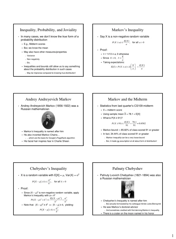
• Andrey Andreyevich Markov (1856-1922) was a

Russian mathematician

• Markov’s Inequality is named after him
• He also invented Markov Chains…
• …which are the basis for Google’s PageRank algorithm
• His facial hair inspires fear in Charlie Sheen

Markov and the Midterm

• Statistics from last quarter’s CS109 midterm
• X = midterm score
• Using sample mean X = 78.1  E[X]
• What is P(X ≥ 91)?
• Markov bound:  85.82% of class scored 91 or greater
• In fact, 34.44% of class scored 91 or greater
• Markov inequality can be a very loose bound
• But, it made no assumption at all about form of distribution!

8582 . 91 1 . 78 91 ] [ ) 91 (     X E X P

Chebyshev’s Inequality

• X is a random variable with E[X] = m, Var(X) = s2
• Proof:
• Since (X – m)2 is non-negative random variable, apply

Markov’s Inequality with a = k2

• Note that: (X – m)2 ≥ k2  |X – m| ≥ k, yielding:

, ) (

2 2

    k k k X P all for s m

2 2 2 2 2 2

] ) [( ) ) (( k k X E k X P s m m     

2 2

) ( k k X P s m   

Pafnuty Chebyshev

• Pafnuty Lvovich Chebyshev (1821-1894) was also

a Russian mathematician

• Chebyshev’s Inequality is named after him
• But actually formulated by his colleague Irénée-Jules Bienaymé
• He was Markov’s doctoral advisor
• And sometimes credited with first deriving Markov’s Inequality
• There is a crater on the moon named in his honor

SLIDE 2

2 Of the Midterm What Say You Chebyshev?

• Statistics from last quarter’s CS109 midterm
• X = midterm score
• Using sample mean X = 78.1  E[X]
• Using sample variance S2 = (24.5)2 = 600.25  s2
• What is P(| X – 78.1 | ≥ 30)?
• Chebyshev bound:  66.69% scored ≥ 108.1 or  48.1
• In fact, 21.85% of class scored ≥ 108.1 or  48.1
• Chebyshev’s inequality is really a theoretical tool

6669 . 900 25 . 600 ) 30 ( ) 30 ] [ (

2 2

     s X E X P 3331 . 6669 . 1 ) 30 ] [ ( 1 ) 30 ] [ (          X E X P X E X P

One-Sided Chebyshev’s Inequality

• X is a random variable with E[X] = 0, Var(X) = s2
• Equivalently, when E[Y] = m and Var(Y) = s2:
• Follows directly by setting X = Y – E[Y], noting E[X] = 0

, ) (

2 2 2

    a a a X P any for s s , ) ] [ (

2 2 2

     a a a Y E Y P any for s s , ) ] [ (

2 2 2

     a a a Y E Y P any for s s

Comments on Midterm, One-Sided One?

• Statistics from last quarter’s CS109 midterm
• X = midterm score
• Using sample mean X = 78.1  E[X]
• Using sample variance S2 = (24.5)2 = 600.25  s2
• What is P(X ≥ 103.1)?
• One-sided Chebyshev bound:  48.99% scored ≥ 103.1
• In fact, 13.26% of class scored ≥ 103.1
• Using Markov’s inequality:

4899 . ) 25 ( 25 . 600 25 . 600 ) 25 1 . 78 (

2 

    X P 7575 . 1 . 103 1 . 78 ) 1 . 103 (    X P

Chernoff Bound

• Say we have MGF, M(t), for a random variable X
• Chernoff bounds:
• Bounds hold for t  0, so use t that minimizes e-taM(t)
• Proof:
• X has MGF: M(t) = E[etX]
• Note P(X ≥ a) = P(etX ≥ eta), use Markov’s inequality:
• Similarity for P(X  a) when t < 0

), ( ) (   



t t M e a X P

ta

all for ), ( ) (   



t t M e a X P

ta

all for

), ( ] [ ] [ ) ( ) (       

 

t t M e e E e e e E e e P a X P

ta tX ta ta tX ta tX

all for

Herman Chernoff

• Herman Chernoff (1923-) is an American

mathematician and statistician

• Chernoff Bound is named after him
• And it actually was derived by him!
• He is Professor Emeritus of Applied Mathematics at

MIT and of Statistics at Harvard University

• I do not know if he is a fan of Charlie Sheen

Chernoff’s Feeling (Unit) Normal

• Z is standard normal random variable: Z ~ N(0, 1)
• Moment generating function:
• Chernoff bounds for P(Z ≥ a)
• To minimize bound, minimize: t2/2 – ta
• Differentiate w.r.t. t, and set to 0: t – a = 0  t = a
• Can proceed similarly for t = a < 0 to obtain:
• Compare to:

, ) (

2 / 2 /

2 2

   

 

t e e e a Z P

ta t t ta

all for

2 /

2

) (

t Z

e t M 

t , ) (

2 /

2

   



a e a Z P

a

all for , ) (

2 /

2

   



a t e a Z P

a

all for dx e z Z P z Z P

z x



  

     

2 /

2

2 1 1 ) ( 1 ) ( 

SLIDE 3

3 Chernoff’s Poisson Pill

• X is Poisson random variable: X ~ Poi(l)
• Moment generating function:
• Chernoff bounds for P(X ≥ i)
• To minimize bound, minimize: l(et – 1) – it
• Differentiate w.r.t. t, and set to 0: let – i = 0  et = i/l
• Compare to:

, ) (

) 1 ( ) 1 (

   

   

t e e e i X P

it e it e

t t

all for

l l

) 1 (

) (





t

e X

e t M

l

1 , ) (

) 1 / (

                      

   

l l l l

l l l l

i/ e i e i e e i e i X P

i i i i i

all for ! ) ( i e i X P

i

l

l 

 

Jensen’s Inequality

• If f(x) is a convex function then E[f(x)] ≥ f(E[X])
• f(x) is convex if f’’(x) ≥ 0 for all x
• Intuition: Convex = “bowl”. E.g.: f(x) = x2, f(x) = ex
• if g(x) = -f(x) is convex, then f(x) is concave
• Proof outline: Taylor series of f(x) about m. Be happy.
• Note: E[f(x)] = f(E[X]) only holds when f(x) is a line
• That is when: f’’(x) = 0 for all x

Johan Jensen

• Johan Ludwig William Valdemar Jensen (1859-

1925) was a Danish mathematician

• He derived Jensen’s inequality
• He was president of the Danish Mathematical Society

from 1892 to 1903

• He has more names than Charlie Sheen

A Brief Digression on Utility Theory

• Utility U(x) is “value” you derive from x
• Can be monetary, but often includes intangibles
• E.g., quality of life, life expectancy, personal beliefs, etc.

0.5 Play? $10,000 yes no $20,000 $0 0.5 0.5 Play? U($10,000) yes no U($20,000) U($0) 0.5

Utility Curves

• Utility curve determines your “risk preference”
• Can be different in different parts of the curve
• We’ll talk more about this near the end of the quarter

Utility Dollars

Jensen’s Investment Advice

• Example: risk-taking investor, with two choices:
• Choice 1: Invest money to get return X where E[X] = m
• Choice 2: Invest money to get return m (probability 1)
• Want to maximize utility: u(R), where R is return
• if u(X) convex then E[u(X)] ≥ u(m), so choice 1 better
• If u(X) concave then E[u(X)]  u(m) so choice 2 better
• Convex u  “risk preferring”, concave u  “risk averse”