1 Z-Score Test for Comparing One-sided vs Two-sided Tests Learned - PDF document

Evaluating Inductive Hypotheses • Accuracy of hypotheses on training data is obviously biased since the hypothesis was CS 391L: Machine Learning: constructed to fit this data. Experimental Evaluation • Accuracy must be evaluated on an independent (usually disjoint) test set. • The larger the test set is, the more accurate the measured accuracy and the lower the Raymond J. Mooney variance observed across different test sets. 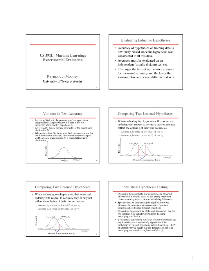University of Texas at Austin 1 2 Variance in Test Accuracy Comparing Two Learned Hypotheses • Let error S ( h ) denote the percentage of examples in an • When evaluating two hypotheses, their observed independently sampled test set S of size n that are incorrectly classified by hypothesis h . ordering with respect to accuracy may or may not • Let error D ( h ) denote the true error rate for the overall data reflect the ordering of their true accuracies. distribution D . – Assume h 1 is tested on test set S 1 of size n 1 • When n is at least 30, the central limit theorem ensures that – Assume h 2 is tested on test set S 2 of size n 2 the distribution of error S ( h ) for different random samples will be closely approximated by a normal (Guassian) distribution. error S2 ( h 2 ) error S 1 ( h 1 ) P( error S ( h )) P( error S ( h )) error S ( h ) error S ( h ) Observe h 1 more accurate than h 2 error D ( h ) 3 4 Comparing Two Learned Hypotheses Statistical Hypothesis Testing • Determine the probability that an empirically observed • When evaluating two hypotheses, their observed difference in a statistic could be due purely to random ordering with respect to accuracy may or may not chance assuming there is no true underlying difference. reflect the ordering of their true accuracies. • Specific tests for determining the significance of the – Assume h 1 is tested on test set S 1 of size n 1 difference between two means computed from two samples gathered under different conditions. – Assume h 2 is tested on test set S 2 of size n 2 • Determines the probability of the null hypothesis , that the two samples were actually drawn from the same error S2 ( h 2 ) underlying distribution. error S 1 ( h 1 ) P( error S ( h )) • By scientific convention, we reject the null hypothesis and say the difference is statistically significant if the probability of the null hypothesis is less than 5% (p < 0.05) or alternatively we accept that the difference is due to an error S ( h ) underlying cause with a confidence of (1 – p). Observe h 1 less accurate than h 2 5 6 1

Z-Score Test for Comparing One-sided vs Two-sided Tests Learned Hypotheses • Assumes h 1 is tested on test set S 1 of size n 1 and h 2 • One-sided test assumes you expected a is tested on test set S 2 of size n 2 . difference in one direction (A is better than • Compute the difference between the accuracy of B) and the observed difference is consistent h 1 and h 2 with that assumption. d = error h − error h ( ) ( ) S 1 S 2 1 2 • Two-sided test does not assume an expected • Compute the standard deviation of the sample difference in either direction. estimate of the difference. error h ⋅ − error h error h ⋅ − error h ( ) ( 1 ( )) ( ) ( 1 ( )) • Two-sided test is more conservative, since it S S S S σ = 1 1 + 2 2 1 1 2 2 d n n requires a larger difference to conclude that 1 2 • Compute the z-score for the difference the difference is significant. d z = σ 7 8 d Z-Score Test for Comparing Sample Z-Score Test 1 Learned Hypotheses (continued) Assume we test two hypotheses on different test sets of size • Determine the confidence in the difference by looking up the highest confidence, C , for the given 100 and observe: = = error h error h ( ) 0 . 20 ( ) 0 . 30 z-score in a table. S S 1 2 1 2 d = error h − error h = − = ( ) ( ) 0 . 2 0 . 3 0 . 1 confidence S S 50% 68% 80% 90% 95% 98% 99% 1 2 1 2 level error h ⋅ − error h error h ⋅ − error h ( ) ( 1 ( )) ( ) ( 1 ( )) S S S S σ = 1 1 + 2 2 z-score 0.67 1.00 1.28 1.64 1.96 2.33 2.58 1 1 2 2 d n n 1 2 ⋅ − ⋅ − 0 . 2 ( 1 0 . 2 ) 0 . 3 ( 1 0 . 3 ) = + = 0 . 0608 100 100 • This gives the confidence for a two-tailed test, for d 0 . 1 z = = = a one tailed test, increase the confidence half way 1 . 644 σ 0 . 0608 d towards 100% − C ( 100 ) Confidence for two-tailed test: 90% ′ C = − ( 100 ) Confidence for one-tailed test: (100 – (100 – 90)/2) = 95% 2 9 10 Sample Z-Score Test 2 Z-Score Test Assumptions • Hypotheses can be tested on different test sets; if Assume we test two hypotheses on different test sets of size same test set used, stronger conclusions might be 100 and observe: error h = error h = ( ) 0 . 20 ( ) 0 . 25 warranted. S S 1 2 1 2 • Test sets have at least 30 independently drawn d = error h − error h = − = ( ) ( ) 0 . 2 0 . 25 0 . 05 S S 1 2 examples. 1 2 error h ⋅ − error h error h ⋅ − error h ( ) ( 1 ( )) ( ) ( 1 ( )) σ = S S + S S • Hypotheses were constructed from independent 1 1 2 2 1 1 2 2 d n n 1 2 training sets. ⋅ − ⋅ − 0 . 2 ( 1 0 . 2 ) 0 . 25 ( 1 0 . 25 ) = + = 0 . 0589 • Only compares two specific hypotheses regardless 100 100 of the methods used to construct them. Does not d 0 . 05 z = = = 0 . 848 compare the underlying learning methods in σ 0 . 0589 d general. Confidence for two-tailed test: 50% Confidence for one-tailed test: (100 – (100 – 50)/2) = 75% 11 12 2

Comparing Learning Algorithms K-Fold Cross Validation • Comparing the average accuracy of hypotheses produced Randomly partition data D into k disjoint equal-sized by two different learning systems is more difficult since subsets P 1 … P k we need to average over multiple training sets. Ideally, we For i from 1 to k do: want to measure: − E error L S error L S ( ( ( )) ( ( ))) Use P i for the test set and remaining data for training S ⊂ D D A D B S i = ( D – P i ) where L X ( S ) represents the hypothesis learned by method L from training data S . h A = L A ( S i ) h B = L B ( S i ) • To accurately estimate this, we need to average over multiple, independent training and test sets. δ i = error Pi ( h A ) – error Pi ( h B ) • However, since labeled data is limited, generally must Return the average difference in error: average over multiple splits of the overall data set into k 1 δ = δ training and test sets. i k ∑ i = 1 13 14 K-Fold Cross Validation Comments Significance Testing • Typically k <30, so not sufficient trials for a z test. • Every example gets used as a test example once and as a training example k –1 times. • Can use ( Student’s ) t-test , which is more accurate when number of trials is low. • All test sets are independent; however, training • Can use a paired t-test, which can determine smaller sets overlap significantly. differences to be significant when the training/sets sets are • Measures accuracy of hypothesis generated for the same for both systems. [( k –1)/ k ] ⋅ |D| training examples. • However, both z and t test’s assume the trials are independent. Not true for k -fold cross validation: • Standard method is 10-fold. – Test sets are independent • If k is low, not sufficient number of train/test – Training sets are not independent trials; if k is high, test set is small and test variance • Alternative statistical tests have been proposed, such as is high and run time is increased. McNemar’s test. • If k =|D|, method is called leave-one-out cross • Although no test is perfect when data is limited and validation. independent trials are not practical, some statistical test that accounts for variance is desirable. 15 16 Sample Experimental Results Learning Curves Which experiment provides better evidence that SystemA is better than SystemB? • Plots accuracy vs. size of training set. • Has maximum accuracy (Bayes optimal) nearly been Experiment 1 Experiment 2 reached or will more examples help? SystemA SystemB Diff SystemA SystemB Diff • Is one system better when training data is limited? • Most learners eventually converge to Bayes optimal given Trial 1 87% 82% +5% Trial 1 90% 82% +8% sufficient training examples. Trail 2 83% 78% +5% Trail 2 93% 76% +17% 100% Bayes optimal +5% –5% Trial 3 88% 83% Trial 3 80% 85% Test Accuracy +10% Trial 4 82% 77% +5% Trial 4 85% 75% – 5% Trial 5 85% 80% +5% Trial 5 77% 82% Random guessing Average 85% 80% +5% Average 85% 80% +5% # Training examples 17 18 3