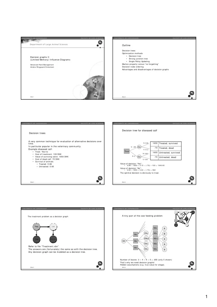
1 Optimization in decision graphs The repeated milk test problem - PDF document

Outline Decision trees Optimization methods • Decision tree Decision graphs II • Strong junction tree (Limited Memory) Influence Diagrams • Single Policy Updating Markov property versus “no forgetting” Advanced Herd Management Decision node ordering Anders Ringgaard Kristensen Advantages and disadvantages of decision graphs Slide 1 Slide 2 Decision tree for diseased calf Decision trees A very common technique for evaluation of alternative decisions over N: 0.88 1650 time. Treated, survived In particular popular in the veterinary community. Y: -100 Die -70 Treated, dead Example diseased calf: Y: 0.12 Treat • Treat: Yes/ no 1650 Untreated, survived N: 0.60 • Cost of treatment: 100 DKK N: 0 • Value of surviving calve: 1650 DKK Die -70 Untreated, dead • Cost of dead calf: 70 DKK Y: 0.40 • Survival of animals: Value of decision “Yes”: • Treated: 0.88 • 0.88 × 1650 + 0.12 × (-70) – 100 = 1343.60 • Untreated: 0.60 Value of decision “No”: • 0.60 × 1650 + 0.40 × (-70) = 962 The optimal decision is obviously to treat. Slide 3 Slide 4 A tiny part of the cow feeding problem The treatment problem as a decision graph Mix R Obs Mix R Me Obs Mix R HS Me Obs Mix R Refer to file “Treatment.xbn” Me Obs Mix The answers are (fortunately) the same as with the decision tree. R Any decision graph can be modeled as a decision tree. Number of leaves: 3 × 4 × 5 × 5 = 300 (only 5 shown) That’s why we need decision graphs! Hidden assumptions (e.g. true value for silage). Slide 5 Slide 6 1

Optimization in decision graphs The repeated milk test problem Unfolding to decision tree The reason for testing the milk from a particular cow is to decide whether or not to pour the milk into the bulk tank: • Only option until Shachter (1986) • If the milk from an infected cow is poured into the bulk tank, the dairy will Influence diagram with “no forgetting” (like the decision tree): reduce the total paym ent by 10% . • Famous article by Jensen, Jensen & Dittmer (1994): • If the milk from the cow is not poured into the bulk tank, the value of that milk is lost. • Strict ordering of nodes • The farmer has 50 cows. • Creation of a “strong” junction tree • Under the action “Pour”: • Implemented in the Hugin software system • The value of the milk (if not infected) is 1000 LImited Memory Influence Diagram (LIMID): • The value of the milk with reduction is 900 • Described by Lauritzen & Nilsson (2001): • Under the action “Don’t pour”: • The value of the milk is 1000 × 49/ 50 = 980 • Decision nodes converted to chance nodes. • It doesn’t matter whether or not the milk is infected • Implemented in the Esthauge LIMID software system Slide 7 Slide 8 As a decision graph Relevant past For a decision made at time t’ the values of all variables observed at time t ≤ t’ are in principle relevant. Moreover, all decisions made at previous time steps t ≤ t’ may be relevant. This observation is referred to, as a “no forgetting” assumption. Requires a strict ordering of the nodes! The result of the test is known when the decision is made. Is that enough? Let’s try! Slide 9 Slide 10 Influence diagrams The decision graph with no forgetting Jensen, Jensen & Dittmer (1994) “No forgetting” assumption: • The value of any previously observed variable is remembered. • Any decision made earlier is remembered. • Graphically, this means that we must insert numerous implicit edges into the net. • Implem ented in the Hugin software system. There are 13 edges into Pour7 ! Slide 11 Slide 12 2

A comparison … Consequences of “no forgetting” The decision strategy found is an optimal one. The optimal strategy gets very complex: Without implicit “no • The optimal decision for Pour7 depends on the value 13 other variables. forgetting” edges. Optimization becomes very demanding from a computational point of view: • Even rather simple decision problems cannot be solved in practice. • The applicational experiences with influence diagrams have been disappointing. • Application to delivery policies in slaughter pigs failed. Implicit “no forgetting” edges visible. Slide 13 Slide 14 LIMIDs – the ideas behind LImited Memory Influence Diagrams Only one decision: Working title: “Demented Influence Diagrams”. • Try the alternatives one by Due to the disappointments with influence diagrams in herd management, one and select the best. a research initiative was initiated: Extend the idea to • Dennis Nilsson as post doc at Aalborg University (later assistant larger nets. professor at LIFE) • Michael Höhle as PhD student at LIFE The goal was to come up with better optimization methods for decision graphs by relaxing the “no forgetting” assumption. Slide 15 Slide 16 Single Policy Updating in LIMIDs Single policy updating in LIMIDs Lauritzen & Nilsson (2001) Usually only near-optimal solutions. Never more complex than a Bayesian network. Not so computationally demanding as influence diagrams. The algorithm may be applied to influence diagrams if all Pour1 Pour3 implicit edges are added. Pour2 Pour5 Pour7 Pour4 Pour6 Rather efficient even for influence diagrams. Implemented in the Esthauge LIMID Software System. Determine an optimization ordering (usually just backwards) Convert all decisions to chance nodes. Update the policy of each decision node one by one. Repeat until convergence. Slide 17 Slide 18 3

Soluble LIMIDs Check for solubility For some LIMIDs, the Single Policy Updating algorithm will provide us with an exact solution. Such LIMIDs are called soluble. All influence diagrams are soluble (i.e. if all implicit edges are added): • Some edges m ay be irrelevant. • The software system can automatically remove irrelevant information edges and find the so-called minimal reduction. • The software system can check whether the minimal reduction is soluble. • If it is soluble, a unique decision node ordering is automatically identified, and only one iteration is necessary. Slide 19 Slide 20 Advantages of decision graphs Disadvantages of decision graphs State space representation: No forgetting: • Variable by variable (as opposed to dynamic • Complexity – hard to solve (even though heavily programming). improved with LIMIDs). • Allow unobservable variables. Only suited for static decision problems: • No forgetting – at least as an option (as opposed to • Time steps must be explicitly modeled (as opposed to dynamic programming). dynamic programming). Only suited for strictly symmetric decision problems (cf irregular decision trees) Slide 21 Slide 22 Properties of methods for decision support Herd constraints Optimization Decision graphs Biological Functional variation limitations Slide 23 Uncertainty Dynamics 4