1 Neutral theory of molecular evolution Motoo Kimura: troubled by - - PDF document

1

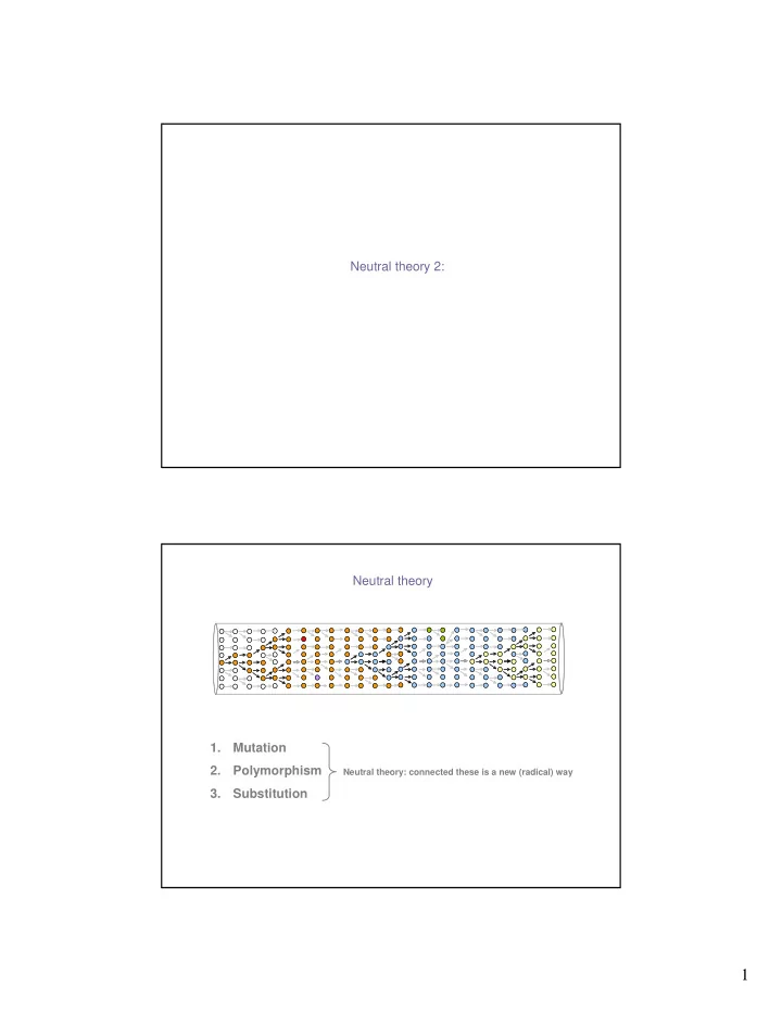
Neutral theory 2: Neutral theory 1. Mutation 2. Polymorphism 3. Substitution

Neutral theory: connected these is a new (radical) way

2

Neutral theory of molecular evolution

Jack King and Thomas Jukes: Independently arrived at same conclusion as Kimura Published (1969) under the provocative title “Non-Darwinian evolution” I cannot over emphasize how radical this idea was at that time. Motoo Kimura:

• troubled by cost Haldane’s dilemma:
• 1 substitution every 300 generations
• troubled by Zukerkandl and Pauling’s (1965) molecular clock:
• 1 substitution every 2 years

Published a model of neutral evolution in 1968

Neutral theory of molecular evolution: elegant simplicity

k = rate of nucleotide substitution at a site per generation [year] k = new mutations × probability of fixation Number of new mutations = µ × 2Ne Probability of fixation = Hence, the neutral rate is: k = µ × 2Ne × 1/2Ne k = µ

e

N 2 1

3

Neutral theory of molecular evolution

Neutral theory: the rate of evolution is independent of effective population size

• mutation-drift equilibrium
• assumes (i) neutrality and (ii) constant mutation rate
• polymorphism is simply a phase of evolution (mutation, polymorphism and

substitution are not separate processes) Evolution by natural selection: k = µ × 4Ne × s

• rate depends on mutation rate and population size and intensity of selection

Remember the genetic drift lecture…

• rate to fixation [under drift] slows with increasing in Ne
• ultimate fate is fixation or loss
• Larger Ne yield larger residence time of a polymorphism in a population

If we run this simulation long enough it will go to fixation of loss; it just takes much longer

4

Ne = 5000 Generations = 30 Generations = 500 Generations = 1000 Generations = 50

Allele frequency

1

t

Ne = small

1

Allele frequency

t

Ne = large

Time to fixation (t) of new alleles in populations with different effective sizes. Note that most new mutations are lost from the population due to drift and those mutations are NOT shown. The time to fixation (as an average) is longer in populations with large size.

A slice in time for each population is shown by a dotted vertical line ( ). Note that at such a slice in time the population with larger effective size is more polymorphic as compared with the smaller population.

The average time to fixation is 4Ne generations

5

Mean time between mutation events (1/µ) is much shorter in the larger population because the number

• f new mutations is on average = µ × 2Ne (for diploid organisms). The mutation rate (µ) is the same in

both populations, but numbers differ because of differences in population size. Allele frequency

1

Ne = small

1

Allele frequency

Ne = large

Mutation event

mean 1/µ mean 1/µ

The average time between neutral substitutions is the reciprocal of µ The population attains an equilibrium substitution rate (k = µ)

k = µ

In words: Large populations: high number of new mutants each generation (2Ne is high) but probability of fixation is low (1/ 2Ne) Small populations: lower number of new mutants each generation (2Ne is lower), but each has a higher probability of fixation (1/ 2Ne is larger)

6

At mutation-drift equilibrium the mutations rate is equal to the substitution rate and the effective population size cancels out. Allele frequency

1

Ne = small: fewer mutations but they drift to fixation more often

1

Allele frequency

Ne = large: more mutations, but few ultimately get fixed

Mutation that goes to fixation (same rate in both populations) Mutation lost due to genetic drift

The population attains an equilibrium substitution rate (k = µ) The population attains an equilibrium polymorphism

He = 4Neµ/(1+4Neµ) θ = 4Neµ

this result assumes an “infinite alleles model” population geneticists are obsessed with the θ parameter

7

Expected equilibrium levels of heterozygosity at a locus as a function of the parameter θ. Heterozygosity will be higher in larger populations. 0.1 0.2 0.3 0.4 0.5 0.6 0.7 0.8 0.9 1 2 4 6 8 10 Heterozygosity (H)

θ

The population attains an equilibrium polymorphism

Neutral theory of molecular evolution

1. The standing level of polymorphism is dependent on effective population size 2. The rate of evolution is independent of effective population size

8

Neutralist-selectionist debate

Neutralists and selectionists actually agree on many points:

• natural selection is ONLY explanation for adaptation
• most new mutations have fitness consequences
• most new mutations are deleterious and subject to purifying selection
• most new mutations are quickly removed from a population by selection
• morphological evolution is mainly driven by selective advantage

Early disagreements focused on genetic load verses selective neutrality:

“It is altogether unlikely that two genes would have identical selective values under all the conditions under which they may coexist in a population. … cases of neutral polymorphism do not exist … it appears probable that random fixation is of negligible evolutionary importance” ⎯Ernst Mayr

Neutral Model

Deleterious Neutral Adaptive

Selectionist Model

Neutralist-selectionist debate: an argument about proportions

9

Misconceptions about neutral theory There has been some confusion about what the neutral theory suggests, so it is worth trying to clear up some of the misconceptions. Myth 1: Only genes that are unimportant can undergo neutral mutations. [Neutral theory only asserts that alternative alleles segregating at a locus are selectively equivalent. Such loci can, and do, encode genes that have important functional roles.] Myth 2: Neutral theory diminished the role of natural selection in adaptation. [To the contrary, neutralists and selectionists both maintain that natural selection is the primary mechanism of adaptation, and that morphological evolution is primarily driven by natural selection.] Myth 3: Nucleotide or amino acid sites that undergo neutral substitutions are not subject to natural

• selection. [Neutral theory does not preclude the possibility that adaptive mutations can occur at sites where neutral

mutations occur. Neutral theory only asserts that adaptive mutations will be much less frequent and will go to fixation much more quickly; hence, most polymorphism observed in a population will be neutral.] Myth 4: Neutral mutations have a selective coefficient of s = 0. [Because natural population sizes are finite, the fate of mildly deleterious alleles can be fixed due to drift. See population genetic Topic 8 for a review.] Myth 5: Neutral mutations are always neutral. [Neutral theory makes no assertions about the stability of the

• environment. The selection coefficient will depend of the environment.]

1. The level of within species genetic variation is determined by population size and mutation rate, and is correlated with the level of sequence divergence between species. 2. The rate of gene evolution (substitution) is inversely related to the level of functional constraint (purifying selection) acting on the gene. [this is macro-evolution] 3. The pattern of base composition at neutral sites reflects mutational equilibrium.

• 4. There is a constant rate of sequence evolution; i.e., a molecular clock.

Predictions of the neutral theory

10

Genetic load and “hard selection”

We already encountered the notion of excess reproductive capacity of a

• species. When excess individuals with the same fitness compete for finite

resources, the resulting mortality is unrelated to natural selection. This is sometimes called “background mortality”. Many models of genetic load were based on Hard Selection. Hard selection refers to any selection-based mortality on top of the mortality that arises when excess individuals have the same fitness; i.e., mortality in addition to the background mortality. All of Kimura’s and Haldane’s arguments concerning genetic load assumed hard selection.

Genetic load and “hard selection”

A question that often comes up: What if we could substitute some of the genetic death for some of the background mortality? Soft selection is the term used to describe the situation when some selective deaths are substituted for non-selective background mortality. The consensus opinion is that natural selection in real populations reflects some mixture of hard and soft selection. Hence, the initial models of genetic load and the cost of selection are thought to

• verestimate the amount of genetic death. Hard and soft selection should be considered extreme
• f a continuum, and natural selection is likely to represent some intermediate point along this

continuum. Do we still need the neutral theory? We will return to this question later.

11

hard and soft selection

20 40 60 80 100 120

1 2

All selective death is substituted with background mortality

Extrem e soft selection

20 40 60 80 100 120

1 2

Mix of soft & hard selection

Only some selective death is substituted with background mortality (50%); some selective death is on top of background mortality (50%) 20 40 60 80 100 120 1 2

Extrem e hard selection

All selective death is

• n top of background

mortality 20 40 60 80 100 120

1 2 Background mortality when all individuals have the same fitness

Background: no selective death

Do we still need the neutral theory? Let’s look at those predictions and see how they fit real data.