1 Consider two loci and 1 generation of random mating: Random - PDF document

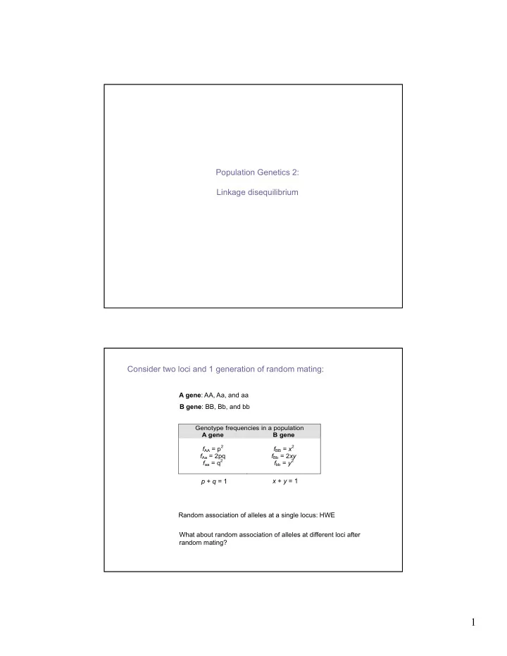
Population Genetics 2: Linkage disequilibrium Consider two loci and 1 generation of random mating: A gene : AA, Aa, and aa B gene : BB, Bb, and bb Genotype frequencies in a population A gene B gene f AA = p 2 f BB = x 2 f Aa = 2pq f Bb = 2 xy f aa = q 2 f bb = y 2 p + q = 1 x + y = 1 Random association of alleles at a single locus: HWE What about random association of alleles at different loci after random mating? 1

Consider two loci and 1 generation of random mating: Random association in gametes Alleles at A locus A( p ) a( q ) Alleles at B locus B AB aB ( x ) ( p x) ( qx ) b Ab ab ( y ) ( py ) ( q y) remember: p + q =1 and x + y = 1 Random association of alleles at a different locus: LINKAGE EQUILIBRIUM GAMETIC PHASE EQUILIBRIUM Consider two loci and 1 generation of random mating: Surprisingly common result: Gene A: HWE Gene B: HWE Gene A + Gene B: disequilibrium 2

Consider two loci (on different chromosomes) and 1 generation of random mating: Example: Population 1: 100% AABB Population 2: 100% aabb Mix populations equally: 50% AABB + 50% aabb 1 generation of random mating (only three matings possible) : AABB x AABB = AABB aabb x aabb = aabb AABB x aabb = AaBb Nine genotypes are possible: AABB AaBB AABb We only see 1/3 after 1 aabb aaBB AAbb generation of random mating! aaBb Aabb AaBb They did not reach equilibrium after one generation of random mating. With continued random mating the “ missing ” genotypes would appear, but not immediately at their equilibrium frequencies! Consider two loci and 1 generation of random mating: - attainment of linkage equilibrium is gradual - about 50% of disequilibrium “ breaks down ” per generation - linkage disequilibrium (LD) persists in populations for many generations - LD = gametic phase disequilibrium 3

LD in individuals (BIOL 2030 stuff): We need a new symbolism Case 1: AB gamete + ab gamete = AaBb Case 2: Ab gamete + aB gamete = AaBb New symbolism: AB/ab indicates the union of AB gamete + ab gamete LD in individuals: Physical linkage: Let ’ s take an AB/ab individual as an example: A B What types of gametes can the AB/ab make? a b By the way, lets assume physical linkage. Notation = AB/ab (1) AB Parental or non-recombinant gametes (2) ab (3) Ab Non-parental or recombinant gametes (4) aB 4

Review meiosis in a single meiocyte: Notation: Gametes Parental (non-recombinant): A B Parental configuration Recombinant: a B Recombinant: A b Parental (non-recombinant): a b 1 crossing over event: 50% parental and 50% recombinant !!! LD in individuals: When genes are on the same chromosome: Physical linkage: A B f AB = f ab ≥ f Ab = f aB a b f (non-recombinant) ≥ f (recombinant) Notation = AB/ab Recombination fraction (r) is the proportion of recombinant gametes produced by an individual. When r = 0: f AB + f ab = 100% [ f Ab + f aB = 0%] When r = 0.5: f AB + f ab = 50% [ f Ab + f aB = 50%] 5

From: i Genetics P. J. Russell (2002) page 350 LD in individuals: When genes are on different chromosomes: Un linked genes: A f AB = f ab = f Ab = f aB a f (non-recombinant) = f (recombinant) B b r = 0.5 • when genes are on different chromosomes • when genes are on same chromosome and recombination is high enough for independent assortment 6

LD in individuals: Individual AB/ab produces the following: (1) AB: f AB = 0.38 (2) ab: f ab = 0.38 (3) Ab: f Ab = 0.12 (4) aB: f aB = 0.12 r = 0.12 + 0.12 = 0.24 What do we expect for individuals if allelic association is random? What do we expect in a population if allelic association is random? LD in populations : Random association in gametes f AB = p x Alleles at A locus f ab = q y A( p ) a( q ) Alleles at B locus f Ab = py B AB aB f aB = qx ( x ) ( p x) ( qx ) b Ab ab ( y ) ( py ) ( q y) f AB + f ab + f Ab + f aB = 1 remember: p + q =1 and x + y = 1 7

LD in populations: The frequency of an AB gamete in a population has two sources: A B A B • Some individuals have this configuration: non-recombinant [parental] • Some individuals produce this as a recombinant configuration. LD in populations:                 non - recombinan ts recombinan ts ' f ( 1 r ) f ( r ) px = − +       AB AB frequency of AB prob of prob of putting probabilit y of gametes in last recomb together A and B no recombinat ion at random from generation recombinan ts 8

                non - recombinan ts recombinan ts ' f ( 1 r ) f ( r ) px = − +       AB AB frequency of AB prob of prob of putting probabilit y of no recombinat ion gametes in last recomb together A and B at random from generation recombinan ts ' f px ( 1 r )( f px ) − = − − Obs. – exp. AB AB D ( 1 r )( f px ) = − − = the linkage disequilibrium parameter AB f AB = p x + D In excess due to LD f ab = q y + D f Ab = py - D Deficient due to LD f aB = qx - D Remember: Individual AB/ab produces the following: (1) AB: f AB = 0.38 (2) ab: f ab = 0.38 (3) Ab: f Ab = 0.12 (4) aB: f aB = 0.12 r = 0.12 + 0.12 = 0.24 What do we expect for an individuals if association is random? What do we expect in a population if association is random? 9

Forces that increase D in populations: 1. Migration 2. Natural selection 3. Genetic Drift LD in populations: • Comparing D among populations is difficult. • Standardize D as a fraction of the theoretical maximum for the popn D D max D f f f f = × − ×           AB ab Ab aB excess due to LD deficient due to LD D qx or py (whichever is smaller) = max 10

LD in a population: Example: blood group polymorphism in a sample of 1000 British people MN blood group Gamete frequencies expected f M = p = 0.5425 MS = 474/2000 = 0.2370 (+) px = 0.1671 D = ef MS × ef ns  − ef Ms × ef nS          f n = q = 0.4575 py = 0.3751 Ms = 611/2000 = 0.3055 (-) non recombinant recombinant qx = 0.1409 nS = 142/2000 = 0.0710 (-) D qx or py = max qy = 0.3166 ns = 773/2000 = 0.3865 (+) Ss blood group f S = x = 0.3080 f s = y = 0.6920 D = (0.2370)(0.3865) – (0.3055)(0.0710) = 0.07 D max : qx = 0.14 or py = 0.37; so D max = 0.14 D is (0.07/0.14)*100 = 50% of the theoretical maximum Homework: Genotype counts in the population Gametes MN locus Ss locus MS = 474 MM = 298 SS = 483 Ms = 611 MN = 489 Ss = 418 NN = 213 ss = 99 NS = 142 Ns = 773 Use chi-square test to: 1. determine if each locus is in HWE 2. determine if gamete frequencies are in equilibrium 11

Recombination reduces LD: Rate of decay of LD under various recombination rates 1 0.9 Standardized disequilibrium r= 0.001 0.8 0.7 0.6 D/Dmax r= 0.01 0.5 0.4 0.3 0.2 0.1 r= 0.1 r= 0.5 0 1 9 17 25 33 41 49 57 65 73 81 89 97 generations Recombination reduces LD: “Hitchhiking” of a mutator gene with and without recombination No recombination r = 0 Recombination r = 0.5 Mutator allele that increase the mutation rate Beneficial allele subject to strong positive selection Adapted from Sniegowski et al. (2000) BioEssays 22:1057-1066. 12

Mapping disease genes: 1. Family studies • Uses family pedigrees • Co-segregation of disease and a marker on the pedigree 2. Allelic association studies (LD mapping) • Uses population data • Relies on strong LD only among closely linked loci • Sample affected and unaffected individuals • Very large samples are required! • Look for markers with more LD in affected individuals Both approached have powers and pitfalls Mapping disease genes: r = 0.01 (1 centiMorgan) is about 1million bp in humans 13

female-limited Batesian mimicry 5-locus linkage group (supergene): § Tail length § Hind-wing pattern § Forewing pattern § Epaulet color § Body color Selection: Only certain complex color Bitter tasting Tasty mimics morphs provide gains in fitness ( Papilio memnon females ) LD: Few maladaptive patterns male produced per generation due to linkage Class I Class III Class II The MHC locus on human chromosome 6 LD over 10s-100s million of bp due to selection for combinations of loci 14

Sexual reproduction reduces LD Linage disequilibrium: Keynotes • Attainment of equilibrium at different loci is gradual; > 1 generation of random mating. • Physical linkage slows the rate to equilibrium even more! • “r” determines the rate to equilibrium, the lower the fraction, the longer to equilibrium. • When r = 0.5 the loci are said to be un-linked; such loci are very far apart on the same chromosome, or in different chromosomes. When r < 0.5 the genes are said to be linked. When r =0 the loci are in permanent disequilibrium. • Disequilibrium can arise from sources other than linkage: o Admixture of populations o Natural selection acting on one or more of the loci o Inbreeding in plants that regularly undergo self-fertilization o Genes located in a chromosomal inversion ( SUPERGENE ) • The term LINKAGE DISEQUILIBRIUM is used to describe any source of disequilibrium, regardless of whether the two genes are physically linked or not. 15