1 Task Level Collaboration with Robotic Assistants Flexible - - PDF document

SLIDE 1

1

Massachusetts Institute of Technology

“Progress Towards Task-Level Collaboration Between Astronauts and Their Robotic Assistants”

Robert Effinger, Andreas Hofmann, Prof. Brian Williams Model-Based Embedded and Robotic Systems Group Massachusetts Institute of Technology

ISAIRAS 2005

(Videos not included in the repository)

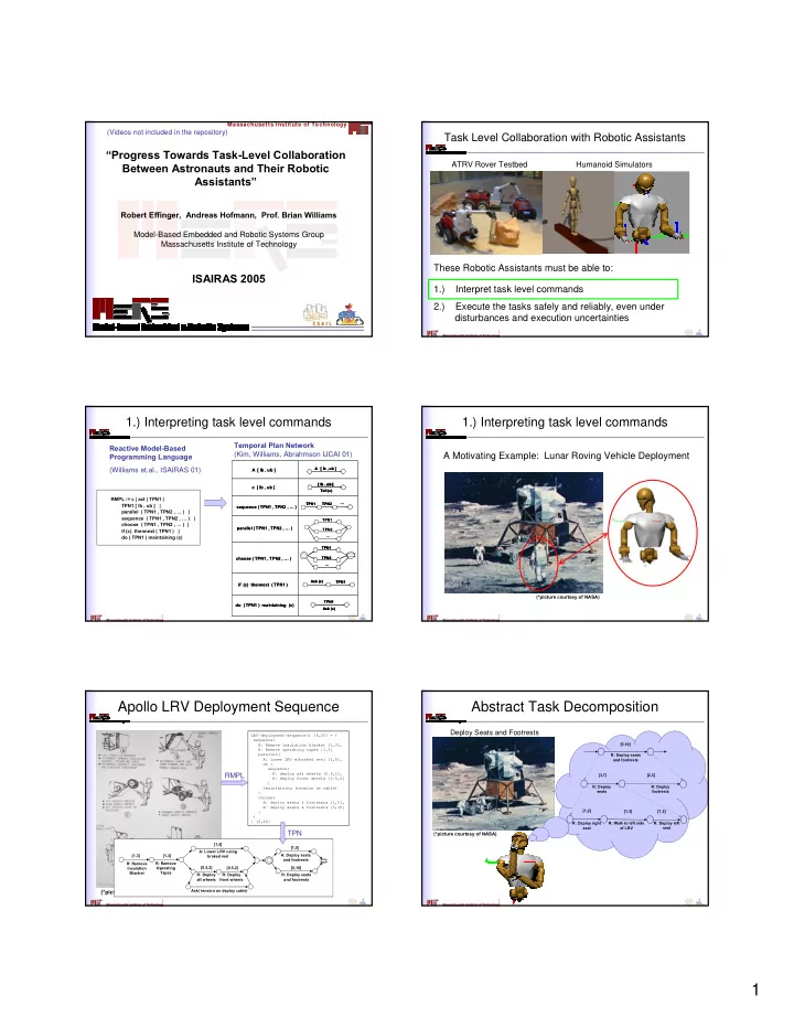
Task Level Collaboration with Robotic Assistants

ATRV Rover Testbed Humanoid Simulators

These Robotic Assistants must be able to: 1.) Interpret task level commands 2.) Execute the tasks safely and reliably, even under disturbances and execution uncertainties

1.) Interpreting task level commands

RMPL := c | act | TPN1 | TPN1 [ lb , ub ] | parallel ( TPN1 , TPN2 , … ) | sequence ( TPN1 , TPN2 , … ) | choose ( TPN1 , TPN2 , … ) | if (c) thennext ( TPN1 ) | do ( TPN1 ) maintaining (c)

Reactive Model-Based Programming Language (Williams et.al., ISAIRAS 01)

A [ lb , ub ]

sequence ( TPN1 , TPN2 , … ) parallel ( TPN1 , TPN2 , … ) choose ( TPN1 , TPN2 , … ) A [ lb , ub ]

TPN1 TPN2 … TPN1 TPN2 … TPN1 TPN2 …

if (c) thennext ( TPN1 ) c [ lb , ub ]

[ lb , ub ] Tell (c) Ask (c) TPN1

do ( TPN1 ) maintaining (c)

TPN1 Ask (c) A [ lb , ub ] A [ lb , ub ]

sequence ( TPN1 , TPN2 , … ) parallel ( TPN1 , TPN2 , … ) choose ( TPN1 , TPN2 , … ) A [ lb , ub ]

TPN1 TPN2 … TPN1 TPN2 … TPN1 TPN2 … TPN1 TPN2 … TPN1 TPN2 …

if (c) thennext ( TPN1 ) c [ lb , ub ]

[ lb , ub ] Tell (c) [ lb , ub ] [ lb , ub ] Tell (c) Ask (c) TPN1 Ask (c) TPN1

do ( TPN1 ) maintaining (c)

TPN1 Ask (c) TPN1 Ask (c)

Temporal Plan Network (Kim, Williams, Abrahmson IJCAI 01)

A Motivating Example: Lunar Roving Vehicle Deployment

(*picture courtesy of NASA)

1.) Interpreting task level commands

Apollo LRV Deployment Sequence

(*picture courtesy of NASA)

LRV-deployment-sequence() [5,20] = { sequence( R: Remove insulation blanket [1,3], R: Remove operating tapes [1,3] parallel( A: Lower LRV w/braked reel [1,5], do ( sequence( R: deploy aft wheels [0.5,2], R: deploy front wheels [0.5,2] ) )maintaining (tension on cable) ) choose( A: deploy seats & footrests [1,5], R: deploy seats & footrests [5,10] ) ) } [5,20] Ask( tension on deploy cable) R: Deploy front wheels R: Deploy aft wheels [0.5,2] R: Remove Insulation Blanket [1,3] R: Remove Operating Tapes [1,3] A: Lower LRV using braked reel [1,5] [0.5,2] A: Deploy seats and footrests R: Deploy seats and footrests [1,5] [5,10]

RMPL TPN

Abstract Task Decomposition

R: Deploy seats and footrests [5,10] R: Deploy seats R: Deploy footrests [3,7] [2,3] R: Deploy left seat R: Walk to left side

• f LRV

R: Deploy right seat [1,2] [1,3] [1,2]

Deploy Seats and Footrests

(*picture courtesy of NASA)

SLIDE 2

2

Task Level Collaboration with Robotic Assistants

ATRV Rover Testbed Humanoid Simulators

These Robotic Assistants must be able to: 1.) Interpret task level commands 2.) Execute the tasks safely and reliably, even under disturbances and execution uncertainties

Flexible Execution Times

Simple Temporal Network (STN): Equivalent Distance Graph Representation: (Dechter, Meiri, Pearl 91)

[ ] l T T u T T u l T T

j i i j i j

− ≤ − ∩ ≤ − ⇒ ∈ − ,

[ ] 5 , 1 ∈ −

i j

T T

Begin- engine-start

[1,5]

End- engine-start

A B

[l,u]

A B

u

• l

STN Distance Graph

Flexible Execution Times

(Dechter, Meiri, Pearl 91)

A B

[1,5]

A B 5

• 1

A Simple STN:

d = 0 d = 5

Consistent !

Determine STN consistency:

• Calculate the Single Source Shortest Path (polynomial-time algorithm)

Flexible Execution Times

Determine STN consistency:

• Calculate the Single Source Shortest Path (polynomial-time algorithm)
• A continually looping negative cycle indicates an inconsistency in STN

(Dechter, Meiri, Pearl 91)

d = 0 d = 1 d = - 4 d = - 3 d = - 8

Inconsistent STN !

Two methods to detect a continually looping negative cycle

1.) Check for any d-value to drop below –nC. 2.) Keep an acyclic spanning tree of support, and terminate when a self-loop is formed. (Cesta, Oddi 96) (most space efficient) (most time efficient)

A Simple STN:

A B

[5,1]

A B 1

• 5

Incremental Reasoning Algorithm

• Basic Idea:

1.) Keep dependency information for each shortest-path value in the distance graph (Cesta, Oddi 96) 2.) Use incremental update rules to localize necessary changes to the distance graph. a.) 3 Update Rules to change a consistent distance graph. b.) 3 Update Rules to repair an inconsistent distance graph.

• ITC’s Novel Claims:

1.) A conflict extraction mechanism to guide plan repair 2.) Allow multiple arc-changes 3.) Can repair inconsistent distance graphs incrementally

Performance Improvements

UAV Scenarios Randomly Generated Plans

Water UAV

NF Z1 NF Z2

WaterA WaterB Fire1 Fire2 Seeker UAV No-Fly Zone

Legend:

Fire Water UAV Base UAV Base

Plan Goal: Extinguish All Fires Vehicles: Two Seeker UAVs One Water UAV Resources: Fuel & Water Comparison of Algorithm Runtime

2 4 6 8 10 12 1 10 19 28 37 46 55 64 73 82 91 Number of Activities Algorithm Runtime (sec) Non-incremental Algorithm Incremental Algorithm

Comparison of Algorithm Runtime

2 4 6 8 10 12 1 10 19 28 37 46 55 64 73 82 91 Number of Activities Algorithm Runtime (sec) Non - incremental Algorithm Incremental Algorithm

SLIDE 3

3

Robustness To Environmental Disturbances and Uncertainty – Andreas Hofmann, PhD Thesis

R: Walk to Right Side

• f LRV

[5,10] R: Walk to Right Side of LRV [5,10]

Qualitative Behavior Specification for Locomotion

Left Foot [t_lb, t_ub] Gait Poses l1 r1 l1 r2 r2 l1 l2 r2 CM Right Foot 1

R CM ∈

start finish right toe-off right heel-strike left toe-off left heel-strike r1 Fwd Lat l1 r2 l2 Foot placement ⎟ ⎠ ⎞ ⎜ ⎝ ⎛ − = K M dt CM d CM CP

tot 2 2

• [Muybridge, 1955]
• Stop-action

photographic study

• f human and

animal motion

• Gaits depicted as

sequences of distinct qualitative poses Flexible spatial and temporal constraints

Nominal Walking

• Angular momentum tightly

conserved during normal walking

20 40 60 80 100 −0.04 −0.02 0.02 Dimensionless Spin Medial−lateral 20 40 60 80 100 −0.01 0.01 Dimensionless Spin Anterior−posterior 20 40 60 80 100 −0.01 0.01 Gait Cycle ( % ) Dimensionless Spin Vertical A

1

y & &

∫ ∫

1

y &

1

y

+

d

k

set

y _

1

+

p

k

• +
• set

y _

1

&

• Allows for linearizing

controllers that decouple state variables and makes them directly controllable

• [Hofmann, et al; 2004]

Walking with constrained foot placement

• When disturbed, sacrifice

tight angular momentum conservation temporarily – Until balance restored

• Implemented in controller

through Lagrangian relaxation

• Orientation goals lower

priority than balance goals Hybrid executive coordinates controllers

• to sequence biped through qualitative state plan

Model-based Executive State Plan MIMO Nonlinear Plant Linearizing Multivariable Controller Plant control inputs Plant state Hybrid Task-level Executive SISO Linear Systems Control parameters Plant state Lf_1 Rf_1 Lf_1 Rf_2 Rf_2 Lf_1 Lf_2 Rf_2

Plan compilation for efficient execution

Model-based Executive State Plan MIMO Nonlinear Plant Linearizing Multivariable Controller Plant control inputs Plant state Hybrid Dispatcher Qualitative Control Plan Plan Compiler SISO Linear Systems Control parameters Plant state

Compiler:

• Computes tubes of feasible control

trajectories from Qualitative State Plan. Dispatcher:

• dynamically searches for optimal

control trajectories within tubes.

• Dispatcher “pulls springs” of each state

variable.

SLIDE 4

4

Qualitative State Plan Goal Regions

lat fwd t l1

[0,0.5] [0,0.5] [0,0.5] [0,0.5] [0,0.5]

[0,1.5] l1 r1 r2 l1 r2 r2 l2 r2 r1 l1 l2 r1 Fwd Lat l1 r2 l2 Foot placement ⎟ ⎠ ⎞ ⎜ ⎝ ⎛ − = K M dt CM d CM CP

tot 2 2

Support polygons

Feasible trajectories must go through goal regions

lat fwd t l1

[0,0.5] [0,0.5] [0,0.5] [0,0.5] [0,0.5]

[0,1.5] l1 r1 r2 l1 r2 r2 l2 r2 r1 l1 l2 r1 Fwd Lat l1 r2 l2 Foot placement ⎟ ⎠ ⎞ ⎜ ⎝ ⎛ − = K M dt CM d CM CP

tot 2 2

Support polygons

Flow tubes denote all feasible trajectories

lat fwd t l1

[0,0.5] [0,0.5] [0,0.5] [0,0.5] [0,0.5]

[0,1.5] l1 r1 r2 l1 r2 r2 l2 r2 r1 l1 l2 r1 Fwd Lat l1 r2 l2 Foot placement ⎟ ⎠ ⎞ ⎜ ⎝ ⎛ − = K M dt CM d CM CP

tot 2 2

Support polygons lat fwd t l1

[0,0.5] [0,0.5] [0,0.5] [0,0.5] [0,0.5]

[0,1.5] l1 r1 r2 l1 r2 r2 l2 r2 r1 l1 l2 r1 Fwd Lat l1 r2 l2 Foot placement ⎟ ⎠ ⎞ ⎜ ⎝ ⎛ − = K M dt CM d CM CP

tot 2 2

Support polygons

Flow tubes denote all feasible trajectories

lat fwd t l1

[0,0.5] [0,0.5] [0,0.5] [0,0.5] [0,0.5]

[0,1.5] l1 r1 r2 l1 r2 r2 l2 r2 r1 l1 l2 r1 Fwd Lat l1 r2 l2 Foot placement ⎟ ⎠ ⎞ ⎜ ⎝ ⎛ − = K M dt CM d CM CP

tot 2 2

Support polygons

Flow tubes denote all feasible trajectories Center of Mass CM tube constrained by foot position tubes:

• Foot positions define

support polygon..

• Center of foot Pressure

CP constrained to be inside support polygon.

• CM coupled to CP.

lat fwd t l1

[0,0.5] [0,0.5] [0,0.5] [0,0.5] [0,0.5]

[0,1.5] l1 r1 r2 l1 r2 r2 l2 r2 r1 l1 l2 r1 Fwd Lat l1 r2 l2 Foot placement ⎟ ⎠ ⎞ ⎜ ⎝ ⎛ − = K M dt CM d CM CP

tot 2 2

Support polygons

SLIDE 5

5

lat fwd t l1

[0,0.5] [0,0.5] [0,0.5] [0,0.5] [0,0.5]

[0,1.5] l1 r1 r2 l1 r2 r2 l2 r2 r1 l1 l2 r1 Fwd Lat l1 r2 l2 Foot placement ⎟ ⎠ ⎞ ⎜ ⎝ ⎛ − = K M dt CM d CM CP

tot 2 2

Support polygons

Center of Mass CM tube constrained by foot position tubes:

• Foot positions define

support polygon..

• Center of foot Pressure

CP constrained to be inside support polygon.

• CM coupled to CP.

lat fwd t l1

[0,0.5] [0,0.5] [0,0.5] [0,0.5] [0,0.5]

[0,1.5] l1 r1 r2 l1 r2 r2 l2 r2 r1 l1 l2 r1 Fwd Lat l1 r2 l2 Foot placement ⎟ ⎠ ⎞ ⎜ ⎝ ⎛ − = K M dt CM d CM CP

tot 2 2

Support polygons

Center of Mass CM tube constrained by foot position tubes:

• Foot positions define

support polygon..

• Center of foot Pressure

CP constrained to be inside support polygon.

• CM coupled to CP.

Successful execution of activity

• Execution successful if trajectory stays in state tube.
• If trajectory begins in initial region, and no disturbances,

will stay in tube.

• If trajectories of each activity stay in tube,

plan executes successfully.

Disturbance displaces trajectory in state space

• If disturbance not too large, displacement stays in tube.
• Activity still executes successfully.

Disturbance displaces trajectory

Disturbance displaces trajectory in state space

• If disturbance too large, trajectory pushed outside tube.
• Goal region not achievable at the required time.
• Plan failure detected immediately leaving more room for

recovery.

Disturbance displaces trajectory

Conclusions

ATRV Rover Testbed Humanoid Simulators These Robotic Assistants must be able to: 1.) Interpret task level commands 2.) Execute the tasks safely and reliably, even under disturbances and execution uncertainties

with the Reactive Model-based Programming Language with Temporal Plan Networks, Qualitative State Plans, and Flow Tubes

SLIDE 6

6

Any Questions? Any Questions? Extra Slides

• Given a consistent STN, changing Arc(i,j)’s cost can

have three possible effects on the shortest path.

1. Arc(i,j) change does not affect the shortest path to node j. 2. Arc(i,j) change improves the shortest path to node j. 3. Arc(i,j) change invalidates the shortest path to node j.

3 Update Rules to Change a Consistent Distance Graph

j i g h E Distance graph

d = 7 d=6 d=5 d=5

2 2 3 10

d = 17 d = shortest path value p = supporting node p = g p = j

• Keep track of the support for each shortest path value

(Cesta & Oddi 96) p = s p = s p = s

CASE 1

3

j i

d=6

g h

2 2 3

d=5 d=5

Distance graph

1.) Arc(i,j) change does not affect shortest path

• The cost from node i to node j increases from 2 to 3.

E

10

d = 7 d = 17 p = g p = j d = shortest path value p = supporting node

• No changes are needed.

p = s p = s p = s

3

CASE 2 j i g h Distance graph

• The cost from node i to node j decreases from 3 to 0.
• Propagate the improved shortest path.

6

i

E

2.) Arc(i,j) change improves shortest path to j

d=6

2 3

d=5 d=5

10

d = 7 d = 17 p = g p = j 16 p = s p = s p = s

SLIDE 7

7

∞

?

4

CASE 3 j i g h

2 3

Distance graph

• Increasing Arc(i,j) now invalidates node j’s shortest path.

E

• Reset node j
• Recursively reset nodes dependent upon node j.
• Insert node j’s parents into the queue so that a new path to node j can be

found for node j and all other invalidated nodes.

3.) Arc(i,j) change invalidates shortest path to j

d=6 d=5 d=5 d = 6 p = i d = 16 p = j

∞

? 7 g 17 j

10

p = s p = s p = s

3 Update Rules to repair an Inconsistent distance graph

• ITC discovers an inconsistency (a negative cycle) by

detecting cyclically dependent backpointers.

D B

2 3

• 1

3 8

• 2
• 2
• 8

d=-3 p=B d=-1 p=A d=-10 p=D

S

2 d=0 p=none

• 1

d=2 p=C

A C

This must be a negative cycle cycle: (A,B,D,C,A)

3 Update Rules to repair an Inconsistent distance graph

• Now ITC must incrementally repair the inconsistency.

D B

2 3

• 1

3 8

• 2
• 2
• 8

d=-3 p=B d=-1 p=A d=-10 p=D

S

2 d=0 p=none

• 1

d=2 p=C

A C

• Three repair steps:

1.) Reset all nodes in negative cycle. 2.) Recursively reset all nodes that depend on the negative cycle nodes. 3.) Put any parent of a reset node that was not also reset on the Q.

Negative cycle: (A,B,D,C,A)

∞ ∞ ∞ ∞

? ? ? ?

3 Update Rules to repair an Inconsistent distance graph

• Now ITC must incrementally repair the inconsistency.

D B

2 3

• 1

3 8

• 2
• 2
• 8

d= ∞ p = ? d= ∞ p= ? d=-10 p=D

S

2 d=0 p=none

• 1

d= ∞ p= ?

A C

• Change arc cost CD to 10.
• Propagate the new shortest path values

Consistent !

5 13 4 2 A B A S

10

Temporal Plan Network ( Kim, Williams, Abrahmson 01 )

p1 p2 p3 pL pR

Redundant Methods

Start End

beHomeBeforeDark() imageTargets( ) driveTo(p3) [0,30] [5,10] [5,10] driveTo(pL) driveTo(p2) driveTo(pR) driveTo(p2) [3,6] [2,5] [20,30] [20,30] [0,0] [0,0]

1

Conflict-Directed Plan Repair

p1 p2 p3 pL pR

Start End

beHomeBeforeDark() imageTargets( ) driveTo(p3) [0,30] [5,10] [5,10] driveTo(pL) driveTo(p2) driveTo(pR) driveTo(p2) [3,6] [2,5] [20,30] [20,30] [0,0] [0,0]

1

Generate New Candidate Plan Test Candidate Plan For Temporal Consistency Inconsistency Incremental Updates

SLIDE 8

8

Conflict-Directed Plan Repair

p1 p2 p3 pL pR

Start End

beHomeBeforeDark() imageTargets( ) driveTo(p3) [0,30] [5,10] [5,10] driveTo(pL) driveTo(p2) driveTo(pR) driveTo(p2) [3,6] [2,5] [20,30] [20,30] [0,0] [0,0]

1

Consistent !

Generate New Candidate Plan Test Candidate Plan For Temporal Consistency Inconsistency Incremental Updates

Conclusions

• ITC is an incremental shortest path algorithm that can repair

distance graphs incrementally as the plan changes

• ITC’s Novel Claims:

1.) A conflict extraction mechanism 2.) Allow multiple arc-changes at once 3.) Can incrementally repair inconsistent distance graphs

• Shows an order of magnitude improvement over non -

incremental planning

• Applicable to any plan representation that uses disjunctions of

simple temporal constraints.