1 Disease with environmental reservoir (e.g. anthrax) S E I S - - PDF document

SLIDE 1

1

Introduction to infectious disease modelling

Jamie Lloyd-Smith Center for Infectious Disease Dynamics Pennsylvania State University with thanks to Ottar Bjornstad for sharing some slides…

Why do we model infectious diseases?

• 1. Gain insight into mechanisms influencing disease spread, and link

individual scale ‘clinical’ knowledge with population-scale patterns.

• 2. Focus thinking: model formulation forces clear statement of

assumptions, hypotheses.

• 3. Derive new insights and hypotheses from mathematical analysis or

simulation.

• 4. Establish relative importance of different processes and parameters,

to focus research or management effort.

• 5. Thought experiments and “what if” questions, since real experiments

are often logistically or ethically impossible.

• 6. Explore management options.

Note the absence of predicting future trends. Models are highly simplified representations of very complex systems, and parameter values are difficult to estimate. quantitative predictions are virtually impossible.

Following Heesterbeek & Roberts (1995)

Epidemic models: the role of data

Why work with data? Basic aim is to describe real patterns, solve real problems. Test assumptions! Get more attention for your work jobs, fame, fortune, etc influence public health policy Challenges of working with data Hard to get good data sets. The real world is messy! And sometimes hard to understand. Statistical methods for non-linear models can be complicated. What about pure theory? Valuable for clarifying concepts, developing methods, integrating ideas. (My opinion) The world (and Africa) needs a few brilliant theorists, and many strong applied modellers.

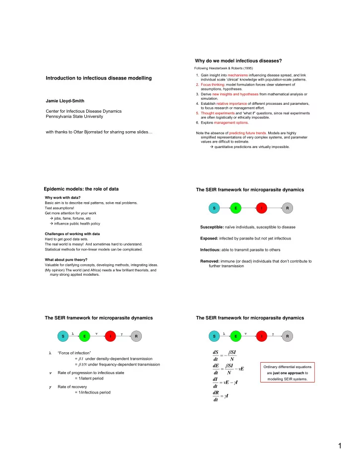
Susceptible: naïve individuals, susceptible to disease Exposed: infected by parasite but not yet infectious Infectious: able to transmit parasite to others Removed: immune (or dead) individuals that don’t contribute to further transmission

The SEIR framework for microparasite dynamics

E I R S

λ “Force of infection” = β I under density-dependent transmission = β I/N under frequency-dependent transmission ν Rate of progression to infectious state = 1/latent period γ Rate of recovery = 1/infectious period

The SEIR framework for microparasite dynamics

E I R γ S λ ν

The SEIR framework for microparasite dynamics

E I R γ S λ ν

I dt dR I E dt dI E N SI dt dE N SI dt dS γ γ ν ν β β = − = − = − =

Ordinary differential equations are just one approach to modelling SEIR systems.

SLIDE 2

2

Depending on time-scale of disease process (and your questions), add host demographic processes.

E I S I R S I S I R S

SEI SIRS SIS

I R S C births deaths

Adapt model framework to disease biology and to your problem! No need to restrict to SEIR categories, if biology suggests otherwise. e.g. leptospirosis has chronic shedding state SICR Vector-borne disease

I R S X Death of pathogen in environment

Disease with environmental reservoir (e.g. anthrax)

IH RH SH IV SV death birth Humans Vectors

Susc Slow Fast ss− ss+

ss− det ss+ det

Rec Susc. Latent Active TB Recovered “Detectable” cases

TB treatment model

Susc Slow Fast ss− ss+

ss− det ss+ det

Rec

TB treatment model

Susc. Latent Active TB Under treatment Recovered

ss+ non-DOTS

Defaulters Tx Completers

Part. rec

Partially recovered Susc Slow Fast ss− ss+

ss− det ss+ det

Rec

Part. rec

TB treatment model

Susc. Latent Active TB

ss+ non-DOTS

Under treatment Susc Slow Fast ss− ss+

ss− det ss+ det

Rec

Part. rec

RN

ss+ DOTS ss+ non-DOTS ss− non-DOTS ss− DOTS

TB treatment model

t t How long does an individual spend in the E compartment? Ignoring further input from new infections:

Residence times

E ν

t

e E t E E dt dE

ν

ν

−

= ⇒ − = ) ( ) (

For a constant per capita rate of leaving compartment, the residence time in the compartment is exponentially distributed.

ODE model Data from SARS

t Divide compartment into n sub-compartments, each with constant leaving rate of ν/n.

Residence times

E1

ν/n

E2 En

ν/n ν/n

…

How to make the model fit the data better?

• “Box-car model” is one modelling trick

t Data from SARS I S λ See Wearing et al (2005) PLoS Med 2: e174 n=40 n=10 n=3 n=1

Residence time is now gamma- distributed, with same mean and flexible variance depending on the number of sub-compartments.

Basic reproductive number, R0

Expected number of cases caused by a typical infectious individual in a susceptible population. R0 ≤ 1 disease dies out R0 > 1 disease can invade Outbreak dynamics

• probability of fade-out
• epidemic growth rate

Disease control

• threshold targets
• vaccination levels

SLIDE 3

3

Calculating R0 – Intuitive approach

× Duration of infectiousness Under frequency-dependent transmission: Rate of infecting others = β S/N = β in wholly susceptible pop’n Duration of infectiousness = 1/recovery rate = 1/γ R0 = β / γ R0 = Per capita rate

• f infecting others

… in a completely susceptible population.

Effective reproductive number

Expected number of cases caused by a typical infectious individual in a population that is not wholly susceptible.

• No. new cases

Time

Epidemic disease: Reff changes as epidemic progresses, as susceptible pool is depleted.

Reff < 1 Reff > 1 Note: Sometimes “effective reproductive number” is used to describe transmission in the presence of disease control measures. This is also called Rcontrol.

Reffective = R0 × S/N Endemic disease: At equilibrium Reff = 1, so that S*/N = 1/R0

Reffective and herd immunity

Reffective = R0 × S/N If a sufficiently high proportion of the population is immune, then Reffective will be below 1 and the disease cannot circulate. The remaining susceptibles are protected by herd immunity. The critical proportion of the population that needs to be immune is determined by a simple calculation:

• For Reff < 1, we need S/N < 1/R0
• Therefore we need a proportion 1-1/R0 to be immune.
• Epidemic threshold

NOTE: not every epidemic threshold parameter is R0!

• Probability of successful invasion
• Initial rate of epidemic growth
• Prevalence at peak of epidemic
• Final size of epidemic (or the proportion of susceptibles

remaining after a simple epidemic)

• Mean age of infection for endemic infection
• Critical vaccination threshold for eradication
• Threshold values for other control measures

What does R0 tell you?

State variables N(t) = Size of host population M(t) = Mean number of sexually mature worms in host population L(t) = Number of infective larvae in the habitat

The basic framework for macroparasite dynamics

L M

For macroparasites the intensity of infection matters! Basic model for a directly-transmitted macroparasite:

death death β infection rate μ death rate of hosts μ1 death rate of adult worms within hosts μ2 death rate of larvae in environment d1 proportion of ingested larvae that survive to adulthood d2 proportion of eggs shed that survive to become infective larvae τ1 time delay for maturation to reproductive maturity τ2 time delay for maturation from egg to infective larva s proportion of offspring that are female

Further complexities: parasite aggregation within hosts and density-dependent effects on parasite reproduction.

The basic framework for macroparasite dynamics

NL L t NM d s dt dL M t L d dt dM β μ τ λ μ μ τ β − − − = + − − =

2 2 2 1 1 1

) ( ) ( ) (

SLIDE 4

4

For macroparasites, R0 is the average number of female offspring (or just

• ffspring in the case of

hermaphroditic species) produced throughout the lifetime of a mature female parasite, which themselves achieve reproductive maturity in the absence of density- dependent constraints on the parasite establishment, survival or reproduction.

R0 for macroparasites

For macroparasites, Reff is the average number of female offspring produced in a host population within which density dependent constraints limit parasite population growth. For microparasites, Reff is the reproductive number in the presence

• f competition for hosts at the population scale.

For macroparasites, Reff is the reproductive number in the presence of competition at the within-host scale. For both, under conditions of stable endemic infection, Reff=1.

Effective R0 for macroparasites Major decisions in designing a model

Even after compartmental framework is chosen, still need to decide: Deterministic vs stochastic Discrete vs continuous time Discrete vs continuous state variables Random mixing vs structured population Homogeneous vs heterogeneous (and which heterogeneities to include?)

Deterministic vs stochastic models

Deterministic models

• Given model structure, parameter values, and initial

conditions, there is no variation in output. Stochastic models incorporate chance.

• Stochastic effects are important when numbers are small,

e.g. during invasion of a new disease

• Demographic stochasticity: variation arising because individual
• utcomes are not certain
• Environmental stochasticity: variation arising from fluctuations in

the environment (i.e. factors not explicitly included in the model)

Important classes of stochastic epidemic models

Monte Carlo simulation

• Any model can be made stochastic by using a pseudo-random

number generator to “roll the dice” on whether events occur. Branching process

• Model of invasion in a large susceptible population
• Allows flexibility in distribution of secondary infections, but

does not account for depletion of susceptibles.

Important classes of stochastic epidemic models

Chain binomial

• Model of an epidemic in a finite population.
• For each generation of transmission, calculates new infected

individuals as a binomial random draw from the remaining susceptibles. Diffusion

• Model of an endemic disease in a large population.
• Number of infectious individuals does a random walk around its

equilibrium value quasi-stationary distribution

SLIDE 5

5

Continuous vs discrete time

Continuous-time models (ODEs, PDEs)

• Well suited for mathematical analysis
• Real events occur in continuous time
• Allow arbitrary flexibility in durations and residence times

Discrete-time models

• Data often recorded in discrete time intervals
• Can match natural timescale of system, e.g. generation

time or length of a season

• Easy to code (simple loop) and intuitive
• Note: can yield unexpected behaviour which may or may

not be biologically relevant (e.g. chaos).

) ( ) 1 ( t N t N λ = + N dt dN λ =

Continuous vs discrete state variables

Continuous state variables arise naturally in differential equation models.

• Mathematically tractable, but biological interpretation is

vague (sometimes called ‘density’ to avoid problem

• f fractional individuals).
• Ignoring discreteness of individuals can yield artefactual

model results (e.g. the “atto-fox” problem).

• Quasi-extinction threshold: assume that population goes

extinct if continuous variable drops below a small value Discrete state variables arise naturally in many stochastic models, which treat individuals (and individual

• utcomes) explicitly.

Models for population structure

Random mixing Multi-group Spatial mixing Network Individual-based model

Population heterogeneities

In real populations, almost everything is heterogeneous – no two individuals are completely alike. Which heterogeneities are important for the question at hand? Do they affect epidemiological rates or mixing? Can parameters be estimated to describe their effect?

• often modelled using multi-group models, but networks, IBMs,

PDEs also useful.

SIR output: the epidemic curve

I dt dR I N SI dt dI N SI dt dS γ γ β β = − = − =

Time Proportion of population

Removed Susceptible Infectious I R S

SIR output: the epidemic curve

Basic model analyses (Anderson & May 1991): Exponential growth rate, r = (R0 − 1)/D Peak prevalence, Imax = 1 − (1+ ln R0)/R0 Final proportion susceptible, f = exp(− R0[1−f]) ≈ exp(−R0)

2 1.778 1.556 1.333 1.111 0.888 9 0.666 7 0.444 4 0.222 2

Time Proportion of population

R0=2 R0=3 R0=5 R0=10

0.2 0.4 0.6 0.8 1

SLIDE 6

6

SIR output: stochastic effects

Time Proportion of population

Removed Susceptible Infectious

Time Proportion of population

Removed Susceptible Infectious

SIR output: stochastic effects

1 2 3 4 5 0.2 0.4 0.6 0.8 1 Basic reproductive number, R0 Probability of extinction

R0

Probability of extinction Time Proportion of population

Stochasticity risk of disease extinction when number of cases is small, even if R0>1.

6 stochastic epidemics with R0=3. Probability of disease extinction following introduction of 1 case.

Cycle period T ≈ 2π (A D)1/2 where A = mean age of infection D = disease generation interval

• r can solve T in terms of SIR model parameters by linearization.

SIR with host demographics: epidemic cycles

Time Proportion of population

I R S births deaths

R I dt dR I N SI dt dI S N SI N dt dS μ γ μ γ β μ β μ − = + − = − − = ) (

110000 120000 130000 140000 20 50 200 1000 5000 Susceptibles Infected

The S-I phase plot

Oct 53 Aug 54 Apr 55 Jan 56 Nov 56 Aug 57 4 8 12 Infected (in thousand) 110 125 140 Susceptible (in thousand)

Summary of simple epidemic patterns

• Absence of recovery: logistic epidemic
• No susceptible recruitment (birth or loss of immunity): simple epidemics
• Susceptible recruitment through birth (or loss of immunity): recurrent

epidemics

Herd immunity and epidemic cycling

The classic example: measles in London

Time Proportion of population

Herd immunity prevents further outbreaks until S/N rises enough that Reff > 1.

SLIDE 7

7

Grenfell et al. (2001)

Herd immunity and epidemic cycling Cycle period depends on the effective birth rate.

Measles in London Baby boom Vaccine era Measles again… Note that measles dies out between major outbreaks in Iceland, but not in the UK or Denmark. What determines persistence of an acute infection? NB: Questions like this are where “atto-foxes” can cause problems.

Persistence and fadeouts

Denmark ~ 5M people UK ~ 60M people Iceland ~ 0.3M people

S I

Intrinsic vs extrinsic forcing – what determines outbreak timing? Untangling the relative roles of intrinsic forcing (population dynamics and herd immunity) and extrinsic forcing (environmental factors and exogenous inputs) is a central problem in population ecology. This is particularly true for ‘outbreak’ phenomena such as infectious diseases or insect pests, where dramatic population events often prompt a search for environmental causes.

8 4 85 8 6 87 8 8 89 9 0 91 9 2 93 9 4 95 9 6 97 98 99 00 01 02 03 04 0 5 06 20 40 60 80 1 00 Number of lepto deaths

Leptospirosis in California sea lions

Intrinsic vs extrinsic forcing – what determines outbreak timing?

Extrinsic factors Pathogen introduction: contact with reservoirs, invasive species, range shifts Climate: ENSO events, warming temperatures Malnutrition: from climate, fisheries or increasing N Pollution: immunosuppressive chemicals, toxic algae blooms Human interactions: Harvesting, protection, disturbance Intrinsic factors Host population size and structure, recruitment rates and herd immunity Example: leptospirosis in California sea lions

Individual “clinical” data

• Latent period: time from infection to transmissibility
• Infectious period: duration (and intensity) of shedding

infectious stages

• Immunity: how effective, and for how long?

Population data

• Population size and structure
• Birth and death rates, survival, immigration and emigration
• Rates of contact within and between population groups

Epidemiological data

• Transmissibility (R0)
• density dependence, seasonality

Data needs I. What’s needed to build a model?

Time series

• Incidence: number of new cases
• Prevalence: proportion of population with disease

Seroprevalence / sero-incidence: shows individuals’ history of exposure. Age/sex/spatial structure, if present. e.g. mean age of infection can estimate R0 Cross-sectional data Seroprevalence survey (or prevalence of chronic disease) endemic disease at steady state insight into mixing epidemic disease outbreak size, attack rate, and risk groups

Data needs II. What’s needed to validate a model?

SLIDE 8

8

Morbidity & Mortality Weekly Report (2003)

Contact tracing

SARS transmission chain, Singapore 2003

Days Cases 5 10 15 20 25 30 35 40 0 1 2 3 4 5 6 7 8 9 101112131415161718192021 Presumed double primaries Presumed within-family transmission

Measles: Latent period 6-9 d, Infectious period 6-7 d, Average serial interval: 10.9 d Observed time intervals between two cases of measles in families of two

• children. Data from Cirencester, England, 1946-1952 (Hope-Simpson 1952)

Household studies Historical mortality records provide data: London Bills of mortality for a week of 1665 Long-term time series

CDC Morbidity and Mortality Weekly Report

Today: several infections are ‘notifiable’

http://www.who.int/research/en/

Outbreak time series

• Journal articles

http://www.who.int/wer/en/

SLIDE 9

9

http://www.cdc.gov/mmwr/ http://www.eurosurveillance.org

Grenfell & Anderson’s (1989) study of whooping cough

Age-incidence

e.g. Walsh (1983) of measles in urban vs rural settings in central Africa

Age-incidence

Dense urban Isolated rural Urban Dense rural Rural

Rubella in Gambia Rubella in UK mumps poliovirus Hepatitis B virus Malaria Age is in years

Age-seroprevalence curves

Seroprevalence: Proportion of population carrying antibodies indicating past exposure to pathogen. Increased transmission leaves signatures in seroprevalence profiles e.g. measles in small (grey) and large (black) families http://www.dcp2.org/pubs/DCP http://www.dcp2.org/pubs/GBD

Two books full of data on important global health problems

• PDF versions free to download.

SLIDE 10

10

Other fields of disease modelling

Within-host models

• pathogen population dynamics and immune response

Other fields of disease modelling

Pathogen evolution

• adaptation to new host species, or evolution of drug resistance

Other fields of disease modelling

Phylodynamics

• how epidemic dynamics interact with pathogen molecular evolution

Community dynamics of disease

Co-infections What happens when multiple parasites are present in the same host? How do they interact? Resource competition? Immune-mediated indirect competition? Facilitation via immune suppression Multiple host species Many pathogens infect multiple species

• when can we focus on one species?
• how can we estimate importance of multi-species effects?

Zoonotic pathogens – many infections of humans have animal reservoirs, e.g. flu, bovine TB, yellow fever, Rift valley fever Reservoir and spillover species Host jumps and pathogen emergence