
SLIDE 1
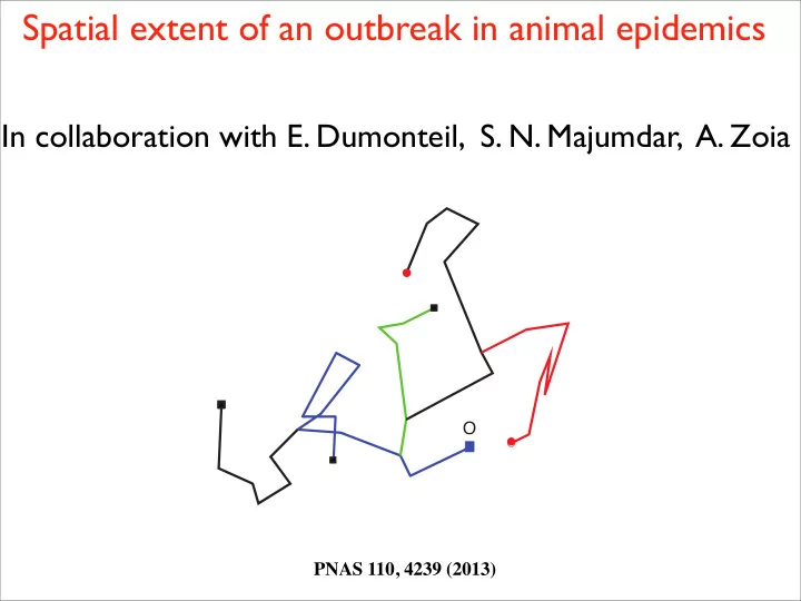
Spatial extent of an outbreak in animal epidemics
In collaboration with E. Dumonteil, S. N. Majumdar, A. Zoia
O
PNAS 110, 4239 (2013)
Spatial extent of an outbreak in animal epidemics In collaboration - - PowerPoint PPT Presentation
Spatial extent of an outbreak in animal epidemics In collaboration with E. Dumonteil, S. N. Majumdar, A. Zoia O PNAS 110, 4239 (2013) SIR model for epidemics Three species : susceptibles (S), infected (I), recovered (R) dS dt = I S
O
PNAS 110, 4239 (2013)
dS dt = −β I S dI dt = β I S − γI dR dt = γI
Three species : susceptibles (S), infected (I), recovered (R) I(t) + S(t) + R(t) = N N being the total population
dS dt = −β I S dI dt = β I S − γI dR dt = γI Initial condition : I(0) = 1, S(0) = N − 1 ≈ N, R(0) = 0 dI dt ' (β N γ) I t ≈ 0, S ≈ N Outbreak regime Reproduction rate: R0 = βN
γ
Reproduction rate: R0 = βN
γ
SIR is a deterministic model. In the outbreak fluctuations are important
O
The good candidate: Brownian process with branching and death
In dt, each infected can:
Problem 1: How to model the space?
Problem 2: How to quantify the area that needs to be quarantined?
O O O
Day 1 Day 2 Day 3
x y x y x y
O
y x M(θ)
C
θ
L = Z 2π M(θ) dθ A = 1 2 Z 2π ⇥ M 2(θ) − (M 0(θ))2⇤ dθ
M(θ) = max
0≤τ≤t [xτ cos θ + yτ sin θ]
M(0) = xτ=tm = xm(t)
M 0(θ = 0) = −xtm sin θ + ytm cos θ|θ=0 = ytm
O
x y x t t y xm y(tm) xm y(tm) tm tm
m(t)i hy2(tm)i
O
x y x t t y xm y(tm) xm y(tm) tm tm
consider a 1d branching process evolving in (0, t)
Qt+dt(xm) = γdt + R0γdtQ2
t(xm) + [1 γ(R0 + 1)]dthQt(xm ∆x)i
Qt(xm) = Proba[global max up to t < xm]
t(xm) + h ∆x2 2 iQ00 t (xm) + . . .
hQt(xm ∆x)i = Qt(xm) + Ddt∂2
xQt(xm) + . . .
hL(t)i = 2π Z ∞ [1 Qt(xm)]dxm. ∂ ∂tQ = D ∂2 ∂x2
m
Q − γ(R0 + 1)Q + γR0Q2 + γ
20 40 60 80 100 101 102 103 104 105 < L(t) > t 10-6 10-5 10-4 10-3 10-2 101 102 Prob(L,t) L
R0=1.15 R0=1 R = 1 . 1 R0=0.99 R0=0.85
10-9 10-8 10-7 10-6 10-5 10-4 10-3 10-2 100 101 102 103 104 Prob(A,t) 500 1000 1500 2000 2500 3000 3500 101 102 103 104 105 < A(t) >
R0=1.15 R0 = 1 R0=1.01 R0=0.99 R0=0.85
500 1000 1500 2000 2500 3000 3500 101 102 103 104 105 < A(t) > t
R0=1.15 R0=1 R0 = 1 . 1 R = . 9 9 R0=0.85
20 40 60 80 100 101 102 103 104 105 < L(t) > t
R0=1.15 R0=1 R = 1 . 1 R0=0.99 R0=0.85
hL(t ! 1)i = 2π s 6D γ + O(t−1/2) hA(t ! 1)i = 24πD 5γ ln t + O(1)
10-9 10-8 10-7 10-6 10-5 10-4 10-3 10-2 100 101 102 103 104 105 106 Prob(A,t) A 10-6 10-5 10-4 10-3 10-2 101 102 103 Prob(L,t) L
When t → ∞ the perimeter remains finite, but the area diverges! How it is possible ? ... Fluctuations Prob(L)
t=∞
− − − − →
L→∞ L−3
Prob(A)
t=∞
− − − − →
A→∞
24πD 5γ A−2
500 1000 1500 2000 2500 3000 3500 101 102 103 104 105 < A(t) > t
R0=1.15 R0=1 R0 = 1 . 1 R = . 9 9 R0=0.85
20 40 60 80 100 101 102 103 104 105 < L(t) > t
R0=1.15 R0=1 R = 1 . 1 R0=0.99 R0=0.85
When R0 6= 1, characteristic time t∗ ⇠ |R0 1|−1. For times t < t∗ the epidemic behaves as in the critical regime. In the subcritical regime, for t > t∗ the epidemic goes to extinction. In the supercritical regime, with probability 1 1/R0 epidemic explodes.
hL(t t∗)i = 4π ✓ 1 1 R0 ◆ p D γ (R0 1) t hA(t t∗)i = 4π ✓ 1 1 R0 ◆ D γ (R0 1) t2 t∗ ⇠ |R0 1|−1
100 101 102 103 104 105 100 101 102 103 < A(t) > t
R = 2 . 5 R = 1 . 5 R = 1 . 2 5 R0 = 1
101 102 100 101 102 103 < L(t) > t
R = 2 . 5 R0=1.5 R0=1.25 R0=1
1 20 40 60 80 100 120 140 x
t=100 t=200 t=400 t =
∞
10 30 40 x
t = 2 t=400 t =∞
1 − 1 R0
∂ ∂tW = D ∂2 ∂x2
m
W + γ(R0 − 1)W − γR0W 2
Problem 1: How to model the space? Brownian motion is the paradigm of animal migration The population is uniformly distributed At time t = 0 an infected individual appears ... and moves in space while human beings take the plane (even when they are sick)
hA(t)i = π Z ∞ dxm [2xm(1 Qt(xm)) Tt(xm)] Similar calculations allows to express the mean area as: Where the evolution of Tt(xm) is governed by: ∂ ∂tTt + ∂xQt(xm) = D ∂2 ∂x2
m
+ 2γR0Qt − γ (R0 + 1)
L = Z 2π M(θ) dθ A = 1 2 Z 2π ⇥ M 2(θ) − (M 0(θ))2⇤ dθ
m(t)i hy2(tm)i
If the process is rotationally invariant any average is independent of θ