[PDF] - 1 1. Need a hashing function, h(k), that To provide a unique set PDF Document

SLIDE 1

1 Searching

Chapter 9 sections 9.1-9.4.1

Searching

A systematic method for locating a record with a key value kj = K. – successful search – unsuccessful search – exact match query – range query

Maps

A map models a searchable collection
f key-value entries
The main operations of a map are for

searching, inserting, and deleting items

Multiple entries with the same key are

not allowed

Applications:

– address book – student-record database

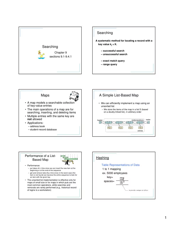
A Simple List-Based Map

We can efficiently implement a map using an

unsorted list

– We store the items of the map in a list S (based

n a doubly-linked list), in arbitrary order
9 c

6 c 5 c 8 c

Performance of a List- Based Map

Performance:

– put takes O(1) time since we can insert the new item at the beginning or at the end of the sequence – get and remove take O(n) time since in the worst case (the item is not found) we traverse the entire sequence to look for an item with the given key

The unsorted list implementation is effective only for

maps of small size or for maps in which puts are the most common operations, while searches and removals are rarely performed (e.g., historical record

f logins to a workstation)

Hashing

Table Representations of Data 1 to 1 mapping

ex. 5000 employees

key= spaces=

to provide a unique set of keys

SLIDE 2

2

To provide a unique set of keys: YOU MUST HAVE A UNIQUE KEY!

ex. binary search ≈ f(n) = 2 log 2 N

2 log2 5000 = 21.6 comparisons O(log2n) How would you like O(1)?

1. Need a hashing function, h(k), that maps key K onto an address in the table.

2. Must ensure that h(k1) ≠ h(k2)

Simple, naïve example: table size = M h(k) = k mod M Example: Table size=7 h(k) = k mod 7

1 2 3 4 5 6

add 10,2,19,14,24,23 10 mod 7 = 3 2 mod 7 = 2

10 2

19 mod 7 = 5

19

Where do 14, 24 and 23 go?

Choosing a Hash Function * a good hash function maps keys

uniformly and randomly – a poor hash function maps keys non-uniformly, or maps contiguous clusters

f keys into clusters of hash table locations.

Example Hash functions

1. Division Method

– choose a prime number as table size, M – interpret keys as integers – h(k) = k mod M

2. Shift Folding

– key is divided into sections – sections are added together – ex. 9 digit key k=013402122 013+402+122 = 537 = h(k) – can use multiplication, subtraction, addition, (whatever) in some fashion, to combine into a final value

SLIDE 3

3

3. Boundary Folding

– like shift folding – every other number is reversed before folding – ex. k = 013402122 013 + 204 + 122 = 339 = h(k) – not much difference – decide which method gives better scattered result based on experiments – used for character codes.

4. Middle Squaring

– take middle portion of key, square it and adjust – ex. k = 013402122 h(k) = 4022 = 161604 adjust - 1) could mod M 2) could take middle 4 digits (6160)

5. Truncation

– simply delete part of the key ε use remaining digits – ex. k = 013402122 h(k) = 122 – easy to compute – not very random ε uniform – seldom used alone - commonly used in conjunction with another method

6. Digit or Character Extraction

– similar to truncation – when key has a predictable value, extract before applying another hash function. – ex. a company coding scheme

7. Random Number Generator

– use key as the “seed” – next number computed is hash value – unlikely 2 different seeds will give the same random number – can be computationally expensive

Collisions ∼∼∼∼∼∼∼

def. h(k1) = h( k2)

recall we need to map keys in a UNIFORM and RANDOM fashion

(For an arbitrary key, any possible table address, 0 to M-1, should be equally likely to be chosen by your hashing function.)

SLIDE 4

4

A BAD EXAMPLE M = 28 = 256 h(k) = k mod M = k mod 256 keys: variable names (registers in assembly) up to 3 characters, use 8-bit ASCII chars

( 1- 24 bit integer, divided into 3 equal 8 bit sections)

Problem with policy - has the effect of selecting the low order character as the value of h(k). K = C3C2C1, numerically K= C325622561+C1*2560 reduced mod 256 has value C1 Hash 6 keys: RX1,RX2,RX3,RY1,RY2,RY3 h(RX1) = h(RY1) = ‘1’ = 49 h(RX2) = h(RY2) = ‘2’ = 50 h(RX3) = h(RY3) = ‘3’ = 51 1) 6 original keys map into only 3 unique addresses 2) contiguous runs of keys, in general, result in contiguous runs of table space How often do collisions really happen? Von Mises Birthday Paradox 23 + people, 50% probability of a match – probe is ∅-1. – Q(n) is probability if you randomly toss n balls into a table with 365 slots, there will be no collision – P(n) = 1- Q(n) probability of a collision – Q(1) = 1 // there will be no collisions

Hashing

Q(2) = Q(1) × (364/365) Q(3) = Q(2) × (363/365) develop a recurrence relation * As soon as the table is 12.9% full, there is greater than a 95% chance that 2 will collide. § Moral of the story§ Even in sparsely occupied hash table, collisions are relatively common. Collision Resolution Policies Open Addressing Inserting keys into other empty locations in the table 1) linear probing – go to next open space – wrap around, if necessary

2) double hashing – calculate a probe decrement P(K) = max (1, K mod M) 3) rehashing – apply h(k) – if a collision, apply h1(k) – if still a collision, apply h2(k) – use entire sequence of hash functions

SLIDE 5

5

Consider a hash

table storing integer keys that handles collision with double hashing

– N = 13 – h(k) = k mod 13 – d(k) = 7 − k mod 7

Insert keys 18, 41,

22, 44, 59, 32, 31, 73, in this order

Example of Double Hashing

1 2 3 4 5 6 7 8 9 10 11 12

1

2 3 4 5 6 7 8 9 10 11 12 k h (k ) d (k )

Collision Resolution Policies

Chaining

use linked lists

Quadratic Collision Processing

– examines locations whose distance form the initial collision point increases as the square of the distance from the previous location tried. – ex. h(k) = A we collide try A+12, A+22, A+32, ... A+R2 – uses wraparound – leaves increasingly larger gaps between successive relocation positions

Load Factors

Suppose table T is of size M, and N entries are occupied, ( M-N are empty) α = N/M load factor of T

ex. M = 100, N = 75, α = 0.75

we say T is 75% full. Clusters def, contiguous runs of occupied entries Primary Clustering * look at linear probing * causes a small “puddle” of keys to form at the collision location. * the small puddle grows larger * the larger it grows, the faster it grows * small puddles connect to form large puddles note - linear probing is subject to primary clustering double hashing is not Secondary Clustering – when any 2 keys have a collision at a given location, they both subsequently examine the same sequence of alternative locations until the collision is resolved. – not as bad as primary clusters – secondary clusters do not form larger secondary clusters – quadratic collision processing is subject to secondary clusters Performance

1) Based on Uniformity and Randomness

f h(k)

2) Based on Collision Resolution Policy 3) Based on Load Factor (Density of Table) “ Density - Dependent Search Technique”

// means you can achieve a highly efficient result if you are willing to waste enough vacant records

SLIDE 6

6

N used M table size

1 1- α

α = (1/2)(1+ ) ave time for successful list accesses (1/2)(1+( )2) unsuccessful

see next page

1 1- α

§ Moral of the story§ THE PERFORMANCE OF A HASH TECHNIQUE IS NOT DEPENDENT ON THE TOTAL NUMBER OF KEYS STORD IN HASH TABLE. PERFORMANCE IS DEPENDENT ON HOW FULL THE TABLE IS.

Deleting items from a hash table 1) can’t just mark empty -- why? 2) want to make reusable Solution: – use a special mark, called a tombstone – allows searches to work correctly – allows insertions to use the spot Good idea to periodically rehash the table.

Dictionary ADT

The dictionary ADT models a

searchable collection of key- element entries

The main operations of a

dictionary are searching, inserting, and deleting items

Multiple items with the same key

are allowed

Applications:

– word-definition pairs – credit card authorizations – DNS mapping of host names (e.g., datastructures.net) to internet IP addresses (e.g., 128.148.34.101)

Dictionary ADT methods:

– find(k): if the dictionary has an entry with key k, returns it, else, returns null – findAll(k): returns an iterator of all entries with key k – insert(k, o): inserts and returns the entry (k, o) – remove(e): remove the entry e from the dictionary – entries(): returns an iterator of the entries in the dictionary – size(), isEmpty()

Hash Table Implementation

We can create a hash-table dictionary

implementation instead of a list-based implementation.

If we use separate chaining to handle collisions,

then each operation can be delegated to a list- based dictionary stored at each hash table cell.

Binary Search

Binary search performs operation find(k) on a dictionary

implemented by means of an array-based sequence, sorted by key

– similar to the high-low game – at each step, the number of candidate items is halved – terminates after a logarithmic number of steps

Example: find(7)
m

l h m l h m l h l=m =h

SLIDE 7

7 What is a Skip List?

A skip list for a set S of distinct (key, element) items is a series of

lists S0, S1 , … , Sh such that

– Each list Si contains the special keys +∞ and −∞ – List S0 contains the keys of S in nondecreasing order – Each list is a subsequence of the previous one, i.e., S0 ⊇ S1 ⊇ … ⊇ Sh – List Sh contains only the two special keys

We show how to use a skip list to implement the dictionary ADT

56 64 78

+∞

31 34 44

−∞

12 23 26

+∞ −∞ +∞

31

−∞

64

+∞

31 34

−∞

23

S0 S1 S2 S3

Search

We search for a key x in a a skip list as follows:

– We start at the first position of the top list – At the current position p, we compare x with y ← key(next(p)) x = y: we return element(next(p)) x > y: we “scan forward” x < y: we “drop down” – If we try to drop down past the bottom list, we return null

Example: search for 78

+∞ −∞

S0 S1 S2 S3

+∞

31

−∞

64

+∞

31 34

−∞

23 56 64 78

+∞

31 34 44

−∞

12 23 26

Randomized Algorithms

A randomized algorithm

performs coin tosses (i.e., uses random bits) to control its execution

It contains statements of the

type

b ← random() if b = 0 do A … else { b = 1} do B …

Its running time depends on

the outcomes of the coin tosses

We analyze the expected

running time of a randomized algorithm under the following assumptions

– the coins are unbiased, and – the coin tosses are independent

The worst-case running time
f a randomized algorithm is
ften large but has very low

probability (e.g., it occurs when all the coin tosses give “heads”)

We use a randomized

algorithm to insert items into a skip list

To insert an entry (x, o) into a skip list, we use a randomized

algorithm:

– We repeatedly toss a coin until we get tails, and we denote with i the number of times the coin came up heads – If i ≥ h, we add to the skip list new lists Sh+1, … , Si +1, each containing only the two special keys – We search for x in the skip list and find the positions p0, p1 , …, pi of the items with largest key less than x in each list S0, S1, … , Si – For j ← 0, …, i, we insert item (x, o) into list Sj after position pj

Example: insert key 15, with i = 2

Insertion

+∞ −∞

10 36

+∞ −∞

23 23

+∞ −∞ S0 S1 S2 +∞ −∞ S0 S1 S2 S3 +∞ −∞

10 36 23 15

+∞ −∞

15

+∞ −∞

23 15

p0 p1 p2

Deletion

To remove an entry with key x from a skip list, we proceed as

follows:

– We search for x in the skip list and find the positions p0, p1 , …, pi of the items with key x, where position pj is in list Sj – We remove positions p0, p1 , …, pi from the lists S0, S1, … , Si – We remove all but one list containing only the two special keys

Example: remove key 34

−∞ +∞

45 12

−∞ +∞

23 23

−∞ +∞ S0 S1 S2 −∞ +∞ S0 S1 S2 S3 −∞ +∞

45 12 23 34

−∞ +∞

34

−∞ +∞

23 34

p0 p1 p2

Implementation

We can implement a skip list

with quad-nodes

A quad-node stores:

– entry – link to the node prev – link to the node next – link to the node below – link to the node above

Also, we define special keys

PLUS_INF and MINUS_INF, and we modify the key comparator to handle them