1
play

1 Observation error Second finding: Randomness The true daily gains - PDF document

Outline Filtering techniques applied to monitoring of daily gain in slaughter pigs: The Kalman filter Introduction - and other methods Basic monitoring Anders Ringgaard Kristensen Shewart control charts DLM and the Kalman


  1. Outline Filtering techniques applied to monitoring of daily gain in slaughter pigs: The Kalman filter • Introduction - and other methods • Basic monitoring Anders Ringgaard Kristensen • Shewart control charts • DLM and the Kalman filter • Simple case • Seasonality • Online monitoring • Used as input to decision support Slide 1 Slide 2 Average daily gain, slaughter pigs 
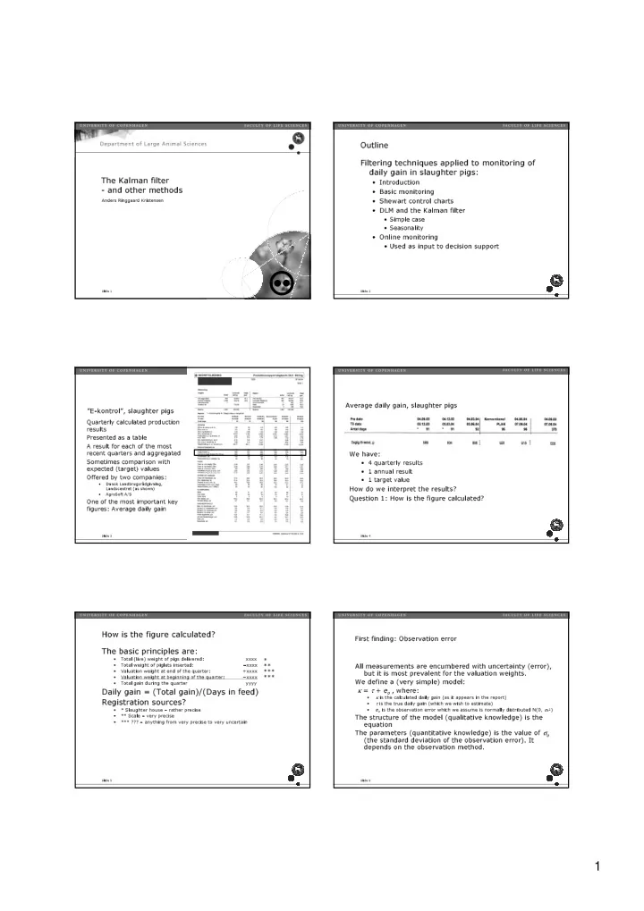
”E-kontrol”, slaughter pigs Quarterly calculated production results Presented as a table A result for each of the most recent quarters and aggregated We have: Sometimes comparison with • 4 quarterly results expected (target) values • 1 annual result Offered by two companies: • 1 target value • Dansk Landbrugsrådgivning, Landscentret (as shown) How do we interpret the results? • AgroSoft A/S Question 1: How is the figure calculated? One of the most important key figures: Average daily gain Slide 3 Slide 4 How is the figure calculated? First finding: Observation error The basic principles are: • Total (live) weight of pigs delivered: xxxx * • Total weight of piglets inserted: −xxxx ** All measurements are encumbered with uncertainty (error), • Valuation weight at end of the quarter: +xxxx *** but it is most prevalent for the valuation weights. • Valuation weight at beginning of the quarter: −xxxx *** We define a (very simple) model: • Total gain during the quarter yyyy κ = τ + e o , where: κ is the calculated daily gain (as it appears in the report) Daily gain = (Total gain)/(Days in feed) • τ is the true daily gain (which we wish to estimate) Registration sources? • e o is the observation error which we assume is normally distributed N(0, σ o 2 ) • * Slaughter house – rather precise • • ** Scale – very precise The structure of the model (qualitative knowledge) is the • *** ??? – anything from very precise to very uncertain equation The parameters (quantitative knowledge) is the value of σ o (the standard deviation of the observation error). It depends on the observation method. Slide 5 Slide 6 1

  2. Observation error Second finding: Randomness The true daily gains τ vary at random. κ = τ + e o , e o ∼ N(0, σ o 2 ) Even if we produce under exactly the same conditions in two τ What we measure is κ successive quarters the results will differ. We shall denote What we wish to know is τ the phenomenon as the “sample error”. We have, τ = θ + e s , where e s is the sample error expressing random variation. We assume e s ∼ N(0, σ s • 2 ) The difference between θ is the underlying permanent (and true) value • the two variables is This supplementary qualitative knowledge should be reflected in the stucture of the model: κ = τ + e o = θ + e s + e o undesired noise κ The parameters of the model are now: σ s og σ o We wish to filter the noise away, i.e. we wish to estimate τ from κ Slide 7 Slide 8 Sample error and measurement error The model in practice: Preconditions The model is necessary for any meaningful interpretation of calculated θ What we measure is κ production results. The standard deviation on the sample error, σ s , depends on the natural What we wish to know is θ individual variation between pigs in a herd and the herd size. The standard deviation of the observation error, σ o , depends on the The difference between the measurement method of valuation weights. For the interpretation of the calculated results, it is the total uncertainty, σ , two variables is undesired τ that matters ( σ 2 = σ s 2 + σ ο noise: 2 ) Competent guesses of the value of σ using different observation methods • Sample noise • Observation noise (1250 pigs): Weighing of all pigs: σ = 3 g • We wish to filter the noise Stratified sample: σ = 7 g • away, i.e. we wish to Random sample: σ = 20 g estimate θ from κ κ • Visual assessment: σ = 29 g • Slide 9 Slide 10 Different observation methods The model in practice: Interpretation Calculated daily gain in a herd was 750 g, whereas the expected target value was 775 g. θ Shall we be worried? It depends on the observation method! A lower control limit (LCL) is the target minus 2 times the standard deviation, i.e. 775 – 2 σ τ Using each of the 4 observation methods, we obtain the following LCLs: • Weighing of all pigs: 775 g – 2 x 3 g = 769 • Stratified sample: 775 g – 2 x 7 g = 761 • Random sample: 775 g – 2 x 20 g = 735 • Visual assessment: 775 g – 2 x 29 g = 717 κ κ κ κ σ = 3 g σ = 7 g σ = 20 g σ = 29 g Slide 11 Slide 12 2

  3. Third finding: Dynamics, time Modeling dynamics Daily gain, slaughter pigs We extend our model to include time. 950 At time n we model the calculated result as follows: κ n = τ sn + e on = θ + e sn + e on 900 850 Only change from before is that we know we have a new result each 800 g 750 quarter. 700 We can calculate control limits for each quarter and plot everything in a 650 diagram: A Shewart Control Chart … 600 θ 2. quarter 97 3. quarter 97 4. quarter 97 1. quarter 98 2. quarter 98 3. quarter 98 4. quarter 98 1. quarter 99 2. quarter 99 3. quarter 99 4. quarter 99 1. quarter 00 2. quarter 00 3. quarter 00 4. quarter 00 1. quarter 01 2. quarter 01 τ 4 … τ 1 τ 2 τ 3 Quarter Daily gain in a herd over 4 years. κ 1 κ 2 κ 3 κ 4 Is this good or bad? Slide 13 Slide 14 A simple Shewart control chart: Weighing all pigs Simple Shewart control chart: Visual assessment Daily gain, slaughter pigs Daily gain, slaughter pigs 950 950 900 900 850 850 800 800 g g 750 750 700 700 650 650 600 600 2. kvartal 97 3. kvartal 97 4. kvartal 97 1. kvartal 98 2. kvartal 98 3. kvartal 98 4. kvartal 98 1. kvartal 99 2. kvartal 99 3. kvartal 99 4. kvartal 99 1. kvartal 00 2. kvartal 00 3. kvartal 00 4. kvartal 00 1. kvartal 01 2. kvartal 01 2. kvartal 97 3. kvartal 97 4. kvartal 97 1. kvartal 98 2. kvartal 98 3. kvartal 98 4. kvartal 98 1. kvartal 99 2. kvartal 99 3. kvartal 99 4. kvartal 99 1. kvartal 00 2. kvartal 00 3. kvartal 00 4. kvartal 00 1. kvartal 01 2. kvartal 01 Period Period Periode Periode Observed gain Expected Observed gain Expected Upper control limit Lower control limit Upper control limit Lower control limit Slide 15 Slide 16 More findings: κ n = θ + e sn + e on Interpretation: Conclusion The true underlying daily gain in the herd, θ , may Something is wrong! Possible explanations: change over time: • The pig farmer has serious problems with fluctuating daily gains. • Trend • Something is wrong with the model: • Seasonal variation • Structure – our qualitative knowledge • Parameters – the quantitative knowledge (standard The sample error e sn may be auto correlated deviations). • Temporary influences The observation error e on is obviously auto correlated: • Valuation weight at the end of Quarter n is the same as the valuation weight at the start of Quarter n +1 Slide 17 Slide 18 3

  4. ”Dynamisk e-kontrol” ”Dynamisk E-kontrol”, results Developed and described by Madsen & Ruby (2000). Principles: • Avoid labor intensive valuation weighing. • Calculate new daily gain every time pigs have been sent to slaughter (typically weekly) • Use a simple Dynamic Linear Model to monitor daily gain κ n = θ n + e sn + e on = θ n + v n , where v n ∼ N(0, σ v 2 ) • θ n = θ n -1 + w n , where w n ∼ N(0, σ w 2 ) • • The calculated results are filtered by the Kalman filter in order to remove random noise (sample error + observation error) Raw data to the left – filtered data to the right Figures from: • Madsen & Ruby (2000). An application for early detection of growth rate changes in the slaughter pig production unit. Computers and Electronics in Agriculture 25, 261-270. Still: Results only available after slaughter Slide 19 Slide 20 F n θ n is the true level The Dynamic Linear Model (DLM) Extending the model described as a vector product. Example A general level, θ 0 n , General, first order Observation equation κ n = θ n + v n , v n ∼ N(0, σ v Observation equation Y t = µ t + v t , v n ∼ N(0, σ v and 4 seasonal effects 2 ) θ 1 n , θ 2 n , θ 3 n and θ 4 n are 2 ) System equation θ n = θ n -1 + w n , w n ∼ N(0, σ w System equation included in the model. µ t = µ t -1 + w n , w n ∼ N(0, σ w 2 ) 2 ) From the model we are able to predict the expected daily gain for next quarter. θ 1 θ 2 θ 3 θ 4 As long as the forecast µ 1 µ 2 µ 3 µ 4 errors are small, production is in control (no large change in τ 1 τ 2 τ 3 τ 4 Y 1 Y 2 Y 3 Y 4 true underlying level)! κ 1 κ 2 κ 3 κ 4 Slide 21 Slide 22 Observed and predicted Analysis of prediction errors Daily gain Daily gain 950 Blue: Observed 900 100 Pink: Predicted 850 80 800 60 g 750 40 700 20 650 g 0 600 -20 -40 7 7 8 8 9 9 0 0 9 9 9 9 9 9 0 0 -60 a l a l a l a l a l a l a l a l r t r t r t r t r t r t r t r t a a a a a a a a -80 v v v v v v v v k k k k k k k k . . . . . . . . -100 2 4 2 4 2 4 2 4 7 7 8 8 9 9 0 0 Quarter 9 9 9 9 9 9 0 0 l l l l l l l l a a a a a a a a r t r t r t r t r t r t t r r t a a a a a a a a v v v v v v v v k k k k k k k k . . . . . . . . 2 4 2 4 2 4 2 4 Quarter Slide 23 Slide 24 4

Download Presentation
Download Policy: The content available on the website is offered to you 'AS IS' for your personal information and use only. It cannot be commercialized, licensed, or distributed on other websites without prior consent from the author. To download a presentation, simply click this link. If you encounter any difficulties during the download process, it's possible that the publisher has removed the file from their server.

Recommend


More recommend