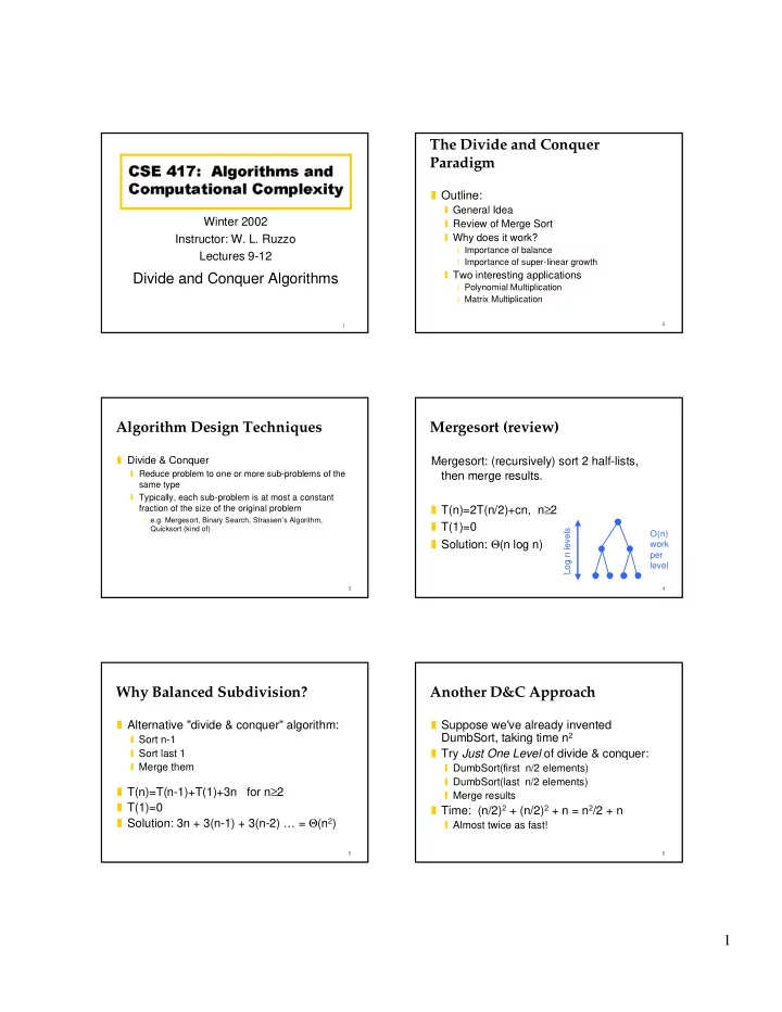
1 Another D&C Approach, cont. Another D&C Approach, cont. - - PDF document

SLIDE 1

1

1

&6($OJRULWKPVDQG &RPSXWDWLRQDO&RPSOH[LW\

Winter 2002 Instructor: W. L. Ruzzo Lectures 9-12

Divide and Conquer Algorithms

2

The Divide and Conquer Paradigm

❚ Outline:

❙ General Idea ❙ Review of Merge Sort ❙ Why does it work?

❘ Importance of balance ❘ Importance of super-linear growth

❙ Two interesting applications

❘ Polynomial Multiplication ❘ Matrix Multiplication

3

Algorithm Design Techniques

❚ Divide & Conquer

❙ Reduce problem to one or more sub-problems of the same type ❙ Typically, each sub-problem is at most a constant fraction of the size of the original problem

❘ e.g. Mergesort, Binary Search, Strassen’s Algorithm, Quicksort (kind of)

4

Mergesort (review)

Mergesort: (recursively) sort 2 half-lists, then merge results. ❚ T(n)=2T(n/2)+cn, n≥2 ❚ T(1)=0 ❚ Solution: Θ(n log n)

Log n levels O(n) work per level

5

Why Balanced Subdivision?

❚ Alternative "divide & conquer" algorithm:

❙ Sort n-1 ❙ Sort last 1 ❙ Merge them

❚ T(n)=T(n-1)+T(1)+3n for n≥2 ❚ T(1)=0 ❚ Solution: 3n + 3(n-1) + 3(n-2) … = Θ(n2)

6

Another D&C Approach

❚ Suppose we've already invented DumbSort, taking time n2 ❚ Try Just One Level of divide & conquer:

❙ DumbSort(first n/2 elements) ❙ DumbSort(last n/2 elements) ❙ Merge results

❚ Time: (n/2)2 + (n/2)2 + n = n2/2 + n

❙ Almost twice as fast!

SLIDE 2

2

7

Another D&C Approach, cont.

❚ Moral 1: Two problems of half size are better than one full-size problem, even given the O(n) overhead

• f recombining, since the base algorithm has

super-linear complexity. ❚ Moral 2: If a little’s good, then more’s better—two levels

• f D&C would be almost 4 times faster, 3 levels

almost 8, etc., even though overhead is

• growing. Best is usually full recursion down to

some small constant size (balancing "work" vs "overhead").

8

Another D&C Approach, cont.

❚ Moral 3: unbalanced division less good:

❙ (.1n)2 + (.9n)2 + n = .82n2/2 + n

❘ The 18% savings compounds significantly if you carry recursion to more levels, actually giving O(nlogn), but with a bigger constant. So worth doing if you can’t get 50-50 split, but balanced is better if you can. ❘ This is intuitively why Quicksort with random splitter is good – badly unbalanced splits are rare, and not instantly fatal.

❙ (1)2 + (n-1)2 + n = n2 - 2n + 2 + n

❘ Little improvement here.

9

Another D&C Example: Multiplying Faster

❚ On the first HW you analyzed our usual algorithm for multiplying numbers

❙ Θ(n2) time

❚ We can do better!

❙ We’ll describe the basic ideas by multiplying polynomials rather than integers ❙ Advantage is we don’t get confused by worrying about carries at first

10

Notes on Polynomials

❙ These are just formal sequences of coefficients so when we show something multiplied by xk it just means shifted k places to the left – basically no work ❙ Usual Polynomial Multiplication: 3x2 + 2x + 2 x2 - 3x + 1 3x2 + 2x + 2

• 9x3 - 6x2 - 6x

3x4 + 2x3+ 2x2 3x4 - 7x3 - x2 - 4x + 2

11

Polynomial Multiplication

❚ Given:

❙ Degree m-1 polynomials P and Q ❘ P = a0 + a1 x + a2 x2 + … + am-2xm-2 + am-1xm-1 ❘ Q = b0 + b1 x+ b2 x2 + … + bm-2xm-2 + bm-1xm-1

❚ Compute:

❙ Degree 2m-2 Polynomial P Q ❙ P Q = a0b0 + (a0b1+a1b0) x + (a0b2+a1b1 +a2b0) x2 +...+ (am-2bm-1+am-1bm-2) x2m-3 + am-1bm-1 x2m-2

❚ Obvious Algorithm:

❙ Compute all aibj and collect terms ❙ Θ (n2) time

12

Naive Divide and Conquer

❚ Assume m=2k

❙ P = (a0 + a1 x + a2 x2 + ... + ak-2 xk-2 + ak-1 xk-1) + (ak + ak+1 x + … + am-2xk-2 + am-1xk-1) xk = P0 + P1 xk ❙ Q = Q0 + Q1 xk ❚ P Q = (P0+P1xk)(Q0+Q1xk) = P0Q0 + (P1Q0+P0Q1)xk + P1Q1x2k ❚ 4 sub-problems of size k=m/2 plus linear combining ❙ T(m)=4T(m/2)+cm ❙ Solution T(m) = O(m2)

SLIDE 3

3

13

Karatsuba’s Algorithm

❚ A better way to compute the terms

❙ Compute

❘ P0Q0 ❘ P1Q1 ❘ (P0+P1)(Q0+Q1) which is P0Q0+P1Q0+P0Q1+P1Q1

❙ Then

❘ P0Q1+P1Q0 = (P0+P1)(Q0+Q1) - P0Q0 - P1Q1

❙ 3 sub-problems of size m/2 plus O(m) work

❘ T(m) = 3 T(m/2) + cm ❘ T(m) = O(mα) where α = log23 = 1.59...

14

Karatsuba: Details

PolyMul(P, Q):

// P, Q are length m =2k vectors, with P[i], Q[i] being // the coefficient of xi in polynomials P, Q respectively. Let Pzero be elements 0..k-1 of P; Pone be elements k..m-1 Qzero, Qone : similar Prod1 = PolyMul(Pzero, Qzero); // result is a (2k-1)-vector Prod2 = PolyMul(Pone, Qone); // ditto Pzo = Pzero + Pone; // add corresponding elements Qzo = Qzero + Qone; // ditto Prod3 = polyMul(Pzo, Qzo); // another (2k-1)-vector Mid = Prod3 – Prod1 – Prod2; // subtract corr. elements R = Prod1 + Shift(Mid, m/2) +Shift(Prod2,m) // a (2m-1)-vector Return( R); Prod1 Mid Prod2 R 2m-1 m m/2

15

Solve: T(n) = 2 T(n/2) + cn

Level Num Size Work 1=20 n cn 1 2=21 n/2 2 c n/2 2 4=22 n/4 4 c n/4 … … … … i 2i n/2i 2i c n/2i … … … … k-1 2k-1 n/2k-1 2k-1 c n/2k-1 k 2k n/2k=1 2k T(1)

16

Solve: T(n) = 4 T(n/2) + cn

... . . . . . .

Level Num Size Work 1=40 n cn 1 4=41 n/2 4 c n/2 2 16=42 n/4 16 c n/4 … … … … i 4i n/2i 4i c n/2i … … … … k-1 4k-1 n/2k-1 4k-1 c n/2k-1 k 4k n/2k=1 4k T(1)

17

Solve: T(1) = c T(n) = 3 T(n/2) + cn

Level Num Size Work 1=30 n cn 1 3=31 n/2 3 c n/2 2 9=32 n/4 9 c n/4 … … … … i 3i n/2i 3i c n/2i … … … … k-1 3k-1 n/2k-1 3k-1 c n/2k-1 k 3k n/2k=1 3k T(1)

... . . . . . .

n = 2k ; k = log2n Total Work: T(n) =

∑ =

k i i i

/ cn 2 3

18

Solve: T(1) = c T(n) = 3 T(n/2) + cn

(cont.)

( ) ( ) ( ) 1

1 2 3 2 3

2 3 1 2 3 0 2 3

− − = ∑ = ∑ = ∑ =

+ = = = k k i i k i i i k i i i

cn cn / cn / cn ) n ( T

( )

1 1 1

1

≠ − − = ∑

+ =

x x x x

k k i i

SLIDE 4

4

19

Solve: T(1) = c T(n) = 3 T(n/2) + cn (cont.)

( ) ( ) ( )

k k k k k

cn cn cn cn 2 3 3 3 2 1 2

2 3 1 2 3 1 2 3

= = <       − =

+ +

20

( ) ( )

a log a log n log n log a log n log

b b b b b b

n b b a = = =

Solve: T(1) = c T(n) = 3 T(n/2) + cn

(cont.)

( ) ( )

... . log n log n log n log

n O n c c n cn cn

n log

59 1 3

2 2 2 2 2

3 3 3 3 3 2 3 3 = = = = =

21

Master Divide and Conquer Recurrence

❚ If T(n)=aT(n/b)+cnk for n>b then

❙ if a>bk then T(n) is ❙ if a<bk then T(n) is Θ(nk) ❙ if a=bk then T(n) is Θ(nk log n)

❚ Works even if it is n/b instead of n/b. ) (

log a

b

n Θ

22

Multiplication – The Bottom Line

❚ Polynomials

❙ Naïve: Θ(n2) ❙ Karatsuba: Θ(n1.59…) ❙ Best known: Θ(n log n)

❘ "Fast Fourier Transform"

❚ Integers

❙ Similar, but some ugly details re: carries, etc. gives Θ(n log n loglog n),

❘ but mostly unused in practice

23

Hints towards FFT:

• I. Interpolation

Given set of values at 5 points

24

Hints towards FFT:

• I. Interpolation

Given set of values at 5 points Find unique degree 4 polynomial going through these points

SLIDE 5

5

25

Hints towards FFT:

• II. Evaluation & Interpolation

P: a0,a1,...,am-1 Q: b0,b1,...,bm-1 P(y0),Q(y0) P(y1),Q(y1) ... P(yn-1),Q(yn-1)

R(y0)=P(y0)Q(y0) R(y1)=P(y1)Q(y1) ... R(yn-1)=P(yn-1)Q(yn-1) R:c0,c1,...,cn-1

∑

= +

←

k j i j i k

b a c

• rdinary polynomial

multiplication Θ(n2) point-wise multiplication

• f numbers O(n)

evaluation at y0,...,yn-1 O(?) interpolation from y0,...,yn-1 O(?)

26

Hints towards FFT:

• III. Evaluation at Special Points

❚ Evaluation of polynomial at 1 point takes O(m), so m points (naively) takes O(m2)—no savings ❚ Key trick: use carefully chosen points where there’s some sharing of work for several points, namely various powers of ❚ Plus more Divide & Conquer. ❚ Result: both eval and interpolation in O(n log n)

1

2

− = = ω

π

i , e

m / i

27

Multiplying Matrices

❚ n3 multiplications, n3-n2 additions

           

• 

          

44 43 42 41 34 33 32 31 24 23 22 21 14 13 12 11 44 43 42 41 34 33 32 31 24 23 22 21 14 13 12 11

b b b b b b b b b b b b b b b b a a a a a a a a a a a a a a a a             + + + + + + + + + + + + + + + + + + + + + + + + + + + + + + + + + + + + =

44 44 34 43 24 42 14 41 42 44 32 43 22 42 12 41 41 44 31 43 21 42 11 41 44 34 34 33 24 32 14 31 42 34 32 33 22 32 12 31 41 34 31 33 21 32 11 31 44 24 34 23 24 22 14 21 42 24 32 23 22 22 12 21 41 24 31 23 21 22 11 21 44 14 34 13 24 12 14 11 42 14 32 13 22 12 12 11 41 14 31 13 21 12 11 11

b a b a b a b a b a b a b a b a b a b a b a b a b a b a b a b a b a b a b a b a b a b a b a b a b a b a b a b a b a b a b a b a b a b a b a b a b a b a b a b a b a b a b a b a b a b a b a b a

• 28

Multiplying Matrices

           

• 

          

44 43 42 41 34 33 32 31 24 23 22 21 14 13 12 11 44 43 42 41 34 33 32 31 24 23 22 21 14 13 12 11

b b b b b b b b b b b b b b b b a a a a a a a a a a a a a a a a             + + + + + + + + + + + + + + + + + + + + + + + + + + + + + + + + + + + + =

44 44 34 43 24 42 14 41 42 44 32 43 22 42 12 41 41 44 31 43 21 42 11 41 44 34 34 33 24 32 14 31 42 34 32 33 22 32 12 31 41 34 31 33 21 32 11 31 44 24 34 23 24 22 14 21 42 24 32 23 22 22 12 21 41 24 31 23 21 22 11 21 44 14 34 13 24 12 14 11 42 14 32 13 22 12 12 11 41 14 31 13 21 12 11 11

b a b a b a b a b a b a b a b a b a b a b a b a b a b a b a b a b a b a b a b a b a b a b a b a b a b a b a b a b a b a b a b a b a b a b a b a b a b a b a b a b a b a b a b a b a b a b a b a

• 29

Multiplying Matrices

           

• 

          

44 43 42 41 34 33 32 31 24 23 22 21 14 13 12 11 44 43 42 41 34 33 32 31 24 23 22 21 14 13 12 11

b b b b b b b b b b b b b b b b a a a a a a a a a a a a a a a a             + + + + + + + + + + + + + + + + + + + + + + + + + + + + + + + + + + + + =

44 44 34 43 24 42 14 41 42 44 32 43 22 42 12 41 41 44 31 43 21 42 11 41 44 34 34 33 24 32 14 31 42 34 32 33 22 32 12 31 41 34 31 33 21 32 11 31 44 24 34 23 24 22 14 21 42 24 32 23 22 22 12 21 41 24 31 23 21 22 11 21 44 14 34 13 24 12 14 11 42 14 32 13 22 12 12 11 41 14 31 13 21 12 11 11

b a b a b a b a b a b a b a b a b a b a b a b a b a b a b a b a b a b a b a b a b a b a b a b a b a b a b a b a b a b a b a b a b a b a b a b a b a b a b a b a b a b a b a b a b a b a b a b a

• 30

Multiplying Matrices

           

• 

          

44 43 42 41 34 33 32 31 24 23 22 21 14 13 12 11 44 43 42 41 34 33 32 31 24 23 22 21 14 13 12 11

b b b b b b b b b b b b b b b b a a a a a a a a a a a a a a a a             + + + + + + + + + + + + + + + + + + + + + + + + + + + + + + + + + + + + =

44 44 34 43 24 42 14 41 42 44 32 43 22 42 12 41 41 44 31 43 21 42 11 41 44 34 34 33 24 32 14 31 42 34 32 33 22 32 12 31 41 34 31 33 21 32 11 31 44 24 34 23 24 22 14 21 42 24 32 23 22 22 12 21 41 24 31 23 21 22 11 21 44 14 34 13 24 12 14 11 42 14 32 13 22 12 12 11 41 14 31 13 21 12 11 11

b a b a b a b a b a b a b a b a b a b a b a b a b a b a b a b a b a b a b a b a b a b a b a b a b a b a b a b a b a b a b a b a b a b a b a b a b a b a b a b a b a b a b a b a b a b a b a b a

• A11

A12 A21 A11B12+A12B22 A22 A11B11+A12B21 B11 B12 B21 B22 A21B12+A22B22 A21B11+A22B21

SLIDE 6

6

31

Multiplying Matrices

❚ T(n)=8T(n/2)+4(n/2)2=8T(n/2)+n2

❙ 8>22 so T(n) is

A11 A12 A21 A11B12+A12B22 A22 A11B11+A12B21 B11 B12 B21 B22 A21B12+A22B22 A21B11+A22B21 =

) ( ) ( ) (

3 log log

n n n

8 a

2 b

Θ = Θ = Θ

32

Strassen’s algorithm

❚ Strassen’s algorithm

❙ Multiply 2x2 matrices using 7 instead of 8 multiplications (and lots more than 4 additions)

❙ T(n)=7 T(n/2)+cn2 ❘ 7>22 so T(n) is Θ(n ) which is O(n2.81)

❙ Fastest algorithms theoretically use O(n2.376) time ❘ not practical but Strassen’s is practical provided calculations are exact and we stop recursion when matrix has size about 100 (maybe 10)

log27

33

The algorithm

❚ P1=A12(B11+B21) P2=A21(B12+B22) ❚ P3=(A11 - A12)B11 P4=(A22 - A21)B22 ❚ P5=(A22 - A12)(B21 - B22) ❚ P6=(A11 - A21)(B12 - B11) ❚ P7= (A21 - A12)(B11+B22) ❚ C11=P1+P3 C12=P2+P3+P6 - P7 ❚ C21= P1+P4+P5+P7 C22=P2+P4

34

Another D&C Example: Fast exponentiation

❚ Power(a,n)

❙ Input: integer n and number a ❙ Output: an

❚ Obvious algorithm

❙ n-1 multiplications

❚ Observation:

❙ if n is even, n=2m, then an=am•am

35

Divide & Conquer Algorithm

❚ Power(a,n) if n=0 then return(1) else x ←Power(a,n/2) if n is even then return(x•x) else return(a•x•x)

36

Analysis

❚ Worst-case recurrence

❙ T(n)=T(n/2)+2

❚ By master theorem

❙ T(n)=O(log n)

❚ More precise analysis:

❙ T(n)= log2n + # of 1’s in n’s binary representation

SLIDE 7

7

37

A Practical Application- RSA

❚ Instead of an want an mod N

❙ ai+j mod N = ((ai mod N)•(aj mod N)) mod N ❙ same algorithm applies with each x•y replaced by

❘ ((x mod N)•(y mod N)) mod N

❚ In RSA cryptosystem (widely used for security)

❙ need an mod N where a, n, N each typically have 1024 bits ❙ Power: at most 2048 multiplies of 1024 bit numbers ❘ relatively easy for modern machines ❙ Naive algorithm: 21024 multiplies

38

Another Example: Binary search for roots (bisection method)

❚ Given:

❙ continuous function f and two points a<b with f(a)<0 and f(b)>0

❚ Find:

❙ approximation to c s.t. f(c)=0 and a<c<b

39

Divide and Conquer Summary

❚ Powerful technique, when applicable ❚ Divide large problem into a few smaller problems of the same type ❚ Choosing subproblems of roughly equal size is usually critical ❚ Examples:

❙ Merge sort, quicksort (sort of), polynomial multiplication, FFT, Strassen’s matrix multiplication algorithm, powering, binary search, root finding by bisection, …