1 The Solution Approach Recognition Framework Model Pictorial - - PDF document

SLIDE 1

1

Efficient Matching of Pictorial Structures

01/30/2007 Pushkala Iyer

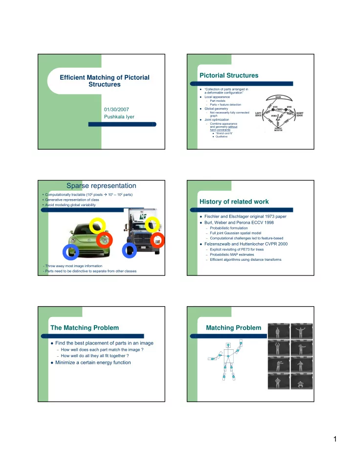
Pictorial Structures

• “Collection of parts arranged in

a deformable configuration”

• Local appearance

–

Part models

–

Parts ≠ feature detection

• Global geometry

–

Not necessarily fully connected graph

• Joint optimization

–

Combine appearance and geometry without hard constraints

“Stretch and fit” Qualitative

Sparse representation

+ Computationally tractable (105 pixels 101 -- 102 parts) + Generative representation of class + Avoid modeling global variability + Success in specific object recognition

• Throw away most image information
• Parts need to be distinctive to separate from other classes

History of related work

Fischler and Elschlager original 1973 paper Burl, Weber and Perona ECCV 1998

– Probabilistic formulation – Full joint Gaussian spatial model – Computational challenges led to feature-based

Felzenszwalb and Huttenlocher CVPR 2000

– Explicit revisiting of FE73 for trees – Probabilistic MAP estimates – Efficient algorithms using distance transforms

The Matching Problem

Find the best placement of parts in an image

– How well does each part match the image ? – How well do all they all fit together ?

Minimize a certain energy function

Matching Problem

SLIDE 2

2

The Solution Approach

• Pictorial Structure model [EF73]
• Restrictions on relationships

–

Tree structure

–

Natural skeletal structure of many animate objects

–

Dynamic programming

• Pairwise relationships

–

Broad range of objects

–

Generalized Distance Transforms

• Globally best match of generic objects
• FH2000 vs other approaches

–

Perona et al – central coordinate system, limited to one articulation point.

–

No hard decisions.

–

Valid configurations are not treated as being equally good.

Recognition Framework Model

Graph Model G = (V, E)

– Parts are the vertices V = {v1, v2, … vn} – If vi, vj are connected, then (vi, vj) є E.

Instance of a part in an image specified by location l.

– Position, Rotation, Scale for 2D parts.

Match cost function mi(I, l) measures how well the

part matches the image I when placed at location l.

Deformation cost function dij(li, lj) for every edge (vi,

vj) measures how well the locations li of vi and lj of vj agree with the object model.

Model Framework

A configuration L = (l1, l2, …,ln) specifies a

location for each of the parts vi in V w.r.t the image.

Best configuration is the configuration that

minimizes the total cost: match cost of individual parts + pair wise cost of the connected pairs of parts.

L* = arg minL (∑(vi,vj) є E dij (li,lj) + ∑vi є V mi(I,li))

Problem reduction

Minimization of L* = arg min L (∑(vi,vj) є E dij (li,lj) + ∑vi є V mi(I,li)) is

O(mn)

–

Where m is the number of discrete values for each li and n is the number of vertices in the graph.

–

Markov Random Fields, Dynamic Contour Models (snakes).

Restricted graphs reduce time complexity –

For first order snakes (chain) reduces to O(m2n) from O(mn)

–

Dynamic programming - is a method of solving problems exhibiting the properties of overlapping subproblems and optimal substructure in a way better than naïve methods.(Wikipedia)

–

Memoization and bottom-up approach.

–

Tree structured graphs enable similar reduction to be achieved.

Problem Reduction

• O(m2n) algorithm is not practical – large number of possible locations

for each part.

• Restriction on pairwise cost function dij yields a minimization algorithm

that is O(mn).

• dij (li,lj) = || Tij(li) – Tji(lj) ||

–

dij measures the degree of deformation.

–

Is restricted to be a Norm.

–

A norm is a function which assigns a positive length or size to all vectors in a vector space, other than the zero vector. (wikipedia)

–

Tij and Tji should be invertible, together capture the ideal relative configurations of parts vi and vj.

–

Tij(li) = Tji(lj) => li and lj are ideal locations for vi and vj

–

Tji(lj) should be discretized in a grid.

Efficient Minimization

Dynamic programming to find the

configuration L* = (l1*, ….ln*) that minimizes the cost.

Computation involves n-1 functions, each of

which specifying the best location of one part w.r.t the possible locations of another part.

SLIDE 3

3

Efficient Minimization

• The best location of a leaf node vj (6)

can be computed as a function of the location of just its parent vi (5).

• Only contribution of lj to the energy is

dij(li,lj) + mj(I,lj) – the contribution of the edge (5,6) and the position of 6.

• Best location of vj given location li of

vi is Bj(li) = min lj (dij(li,lj) + mj(I, lj))

• Replacing min by argmin, we get the

best location of vj as a function of the location li of its parent vi.

Efficient Minimization

For non leaf vertices vj ≠ vr, if Bc(lj)

is known for every child vc є of Cj, then the best location of vj given its parent vi is Bj(li) = min lj (dij(li, lj) + mj(I,lj) + ∑ vc є Cj Bc(lj))

Replacing min with arg-min yeilds

the best location of vj as a function

• f li.

Efficient Minimization

For the root node vr, if Bc(lr) is

known for every child vc є Cr, then the best location of the root is Lr* = arg min lr (mr(I, lr) + ∑ vc є Cr Bc(lj))

Algorithm

Recursive equations specify an algorithm. For every leaf node, compute its best location as a function of

the location of its parent.

For every non leaf node X, compute its best location as a

function of the location of X’s parent, also taking into consideration the cost of placing X’s children (previous step).

Repeat until the best location of the root is calculated. Now traverse the tree starting at the root, to find the optimum

configuration.

O(nM) – n (# nodes) M (time to compute Bj(li ) and B’j(li))

Distance Transforms

• A distance transform, also

known as distance map or distance field, is a representation of a digital

• image. (Wikipedia)
• The map supplies each pixel of

the image with the distance to the nearest obstacle pixel. A most common type obstacle pixel is a boundary pixel in a binary image.

• An example of a chessboard

distance transform on a binary image.

Generalized Distance Transforms

• DB(Z) = min w є B || z- w || where B is a subset of G
• DB(Z) = min w є G (|| z- w || + 1B (w)) where 1B (w) is an indicator function for membership in

B.

• Algorithm (G.Borgefors) computes this in O(mD) time for a D dimensional grid.
• Two pass, local neighborhoods of 7x7 pixels used.
• Meijster, Roerdink & Hesselink:
• Generic distance transform algorithm in linear time.
• 2 Phases, first columnwise, second rowwise, each phase 2 scans.
• Per row computation independent of per column computation, can be parallelized.
• Df(Z) = min w є G (|| z- w || + f(w))
• How that helps:
• Given dij (li,lj) = || Tij(li) – Tji(lj) ||
• Bj(li) = Df(Tij(li)) where f(w) = mj(I, Tji
• 1(w)) +∑ Tji
• 1(w))

SLIDE 4

4

Computation

• D is 4 (x, y, rotation, scale)
• D[x,y,θ,s] is initialized to the values of function f(w)
• D[x,y,θ,s] = min(D[x, y, θ,s],

D[x-1, y, θ, s] + kx, D[x, y-1, θ, s] + ky, D[x, y, θ-1, s] + kθ, D[x, y, θ, s-1] + ks)

• D[x,y,θ,s] = min(D[x, y, θ,s],

D[x+1, y, θ, s] + kx, D[x, y+1, θ, s] + ky, D[x, y, θ+1, s] + kθ, D[x, y, θ, s+1] + ks)

• Doesn’t consider periodic θ.
• Special handling of boundary cases, additional passes.
• Bj(li) computable in O(m) time.

Person Model

Flexible revolute joints. Ideal relative orientation given by θij. Deformation cost measures observed

deviation from ideal.

Given the observed locations li = (θi, si, xi, yi)

and lj = (θj, sj, xj, yj)

dij(li, lj) = wij

θ |(θj – θi) – θij|

+ wij

s |(log sj – log si) – log sij|

+ wij

x | x’ij – x’ji|

+ wij

y |y’ij – y’ji|

Large wij

s ,wij x ,wij y and Small wij θ

Recognition Results

Car Model

Flexible prismatic joints dij(li, lj) =

Infinity |(θj – θi)| + wij

s |(log sj – log si) –

log sij| + wij

x | x’ij – x’ji|

+ wij

y |y’ij – y’ji|

Bayesian Formulation

Best match by MAP estimation

L* = arg max L (Pr(L|I))

Applying Bayes rule,

L* = arg max L (Pr(I|L) Pr(L))

Prior information – from spring connections Likelihood – approx product of match qualities for

individual parts.

To minimize the energy function, take the negative

logarithm: L* = arg minL (∑(vi,vj) є E dij (li,lj) - ∑vi є V ln gi(I,li))

Summary

• No decisions until the end.

–

No feature detection

• Quality maps or likelihoods

–

No hard geometric constraints

• Deformation costs or priors
• Efficient algorithms.

–

Dynamic programming critical

–

Not applicable to all problems, need good factorizations of geometry and appearance

• Good for categorical object recognition.

–

Qualitative descriptions of appearance

–

Factoring variability in appearance and geometry

• Deals well with occlusion.

–

In contrast to hard feature detection

• Most applicable to 2D objects defined by relatively small number of parts.
• Unclear how to extend to large number of transformation parameters per part.

–

Explicit representation grows exponentially

• No known way of using to index into model databases.

SLIDE 5

5

References

Efficient Matching of Pictorial Structures – Pedro F

Felzenswalb & Daniel P Huttenlocher

Representation & Matching of Pictorial Structures –

Martin A Fischler & Robert A Elschlager

Discussion of Pictorial Structures - Pedro F

Felzenswalb & Daniel P Huttenlocher

A general algorithm for computing distance

transforms in linear time – A Meijster, J B T M Roerdink and W H Hesselink

Part Based Models – Rob Fergus Wikipedia