] [ ( ) 1 = g u , 0 1 + 2 u e 1 Funzione di - PowerPoint PPT Presentation

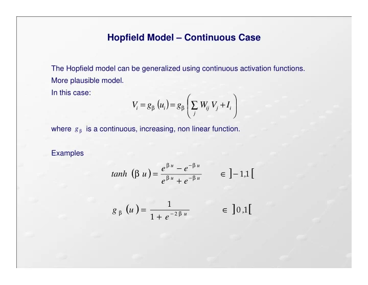
Hopfield Model – Continuous Case The Hopfield model can be generalized using continuous activation functions. More plausible model. In this case:   ( ) = = ∑ +   V g u g W V I β β i i ij j i   j where is a continuous, increasing, non linear function. g β Examples β − β − u u ] [ ( ) e e β = ∈ − tanh u 1 , 1 β − β + u u e e ] [ ( ) 1 = ∈ g u , 0 1 β − β + 2 u e 1

Funzione di attivazione +1 ß > 1 ß = 1 ß < 1 -1 ( ) ( ) = β f x tanh x

Updating Rules Several possible choices for updating the units : Asynchronous updating: one unit at a time is selected to have its output set Synchronous updating: at each time step all units have their output set Continuous updating: all units continuously and simultaneously change their outputs

Continuous Hopfield Models Using the continuous updating rule, the network evolves according to the following set of (coupled) differential equations:   dV ( ) τ = − + = − + ∑ +   i V g u V g w V I β β i i i i ij j i   dt j τ τ where are suitable time constants ( > 0). i i ∀ i Note When the system reaches a fixed point ( dV dt / = 0 ) we get i ( ) = V g u β i i Indeed, we study a very similar dynamics ( ) du τ = − + + ∑ i u w g u I β i i ij j i dt j

Modello di Hopfield continuo (energia) dV dE dV ( ) dV dV 1 1 − = − − + − ∑ ∑ ∑ ∑ j 1 i i i T V T V g V I β ij j ij i i i dt dt dt dt dt 2 2 ij ij i i   dV = − ∑ ∑ − +   i T V u I ij j i i   dt i j dV du = − τ ∑ i i i dt dt i 2   ( ) du ′ = − τ ≤ ∑   i g u 0 β i i   dt i τ > g Perché è monotona crescente e . 0 β i dE du = ⇔ = N.B. i 0 0 dt dt u cioè è un punto di equilibrio i

The Energy Function As the discrete model, the continuous Hopfield network has an “energy” function, provided that W = W T : ( ) 1 − = − + − ∑∑ ∑ ∫ ∑ V i 1 E w V V g V dV I V β ij i j i i 0 2 i j i i Easy to prove that dE ≤ 0 dt with equality iff the net reaches a fixed point.

Modello di Hopfield continuo (relazione con il modello discreto) Esiste una relazione stretta tra il modello continuo e quello discreto. Si noti che : ( ) ( ) ( ) = = β ≡ β V g u g u g u β i i i i 1 ( ) 1 − = β 1 u g V quindi : i i Il 2 o termine in E diventa : V i ( ) dV 1 − ∑ ∫ 1 g V β i i 0 L’integrale è positivo (0 se V i =0). β → ∞ Per il termine diventa trascurabile, quindi la funzione E del modello continuo diventa identica a quello del modello discreto

Optimization Using Hopfield Network § Energy function of Hopfield network 1 = − − ∑ ∑ ∑ E w V V I V ij i j i i 2 i j i § The network will evolve into a (locally / globally) minimum energy state § Any quadratic cost function can be rewritten as the Hopfield network Energy function. Therefore, it can be minimized using Hopfield network. § Classical Traveling Salesperson Problem (TSP) § Many other applications • 2-D, 3-D object recognition • Image restoration • Stereo matching • Computing optical flow