1/31/2007 Massachusetts Institute of Technology Context Model - PDF document

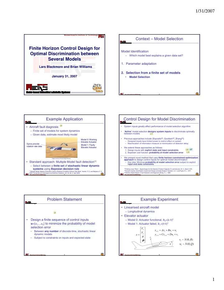
1/31/2007 Massachusetts Institute of Technology Context – Model Selection Finite Horizon Control Design for Model Identification Optimal Discrimination between – Which model best explains a given data set? Several Models 1. Parameter adaptation Lars Blackmore and Brian Williams 2. Selection from a finite set of models January 31, 2007 • Model Selection 2 Example Application Control Design for Model Discrimination L3 • System inputs greatly affect performance of model selection algorithm • Aircraft fault diagnosis – Finite set of models for system dynamics • ‘Active’ model selection designs system inputs to discriminate optimally between models – Given data, estimate most likely model L11 • Previous approaches include (Esposito [2] , Goodwin [3] , Zhang [4] ) Model 0: Working – Designed inputs have limited power to restrict effect on system Elevator Actuator – Maximization of information measure or minimization of detection delay Gyros provide Model 1: Faulty rotation rate data Elevator Actuator • We extend these approaches as follows: LB7 1. Design inputs with explicit state and input constraints L12 2. Bayesian cost function: probability of model selection error L13 • We present novel method that uses finite horizon constrained optimization Image courtesy of Aurora Flight Sciences approach to design control inputs for optimal model discrimination • Standard approach: Multiple Model fault detection [1] – Key idea: Minimise probability of model selection error subject to explicit input and state constraints – Select between a finite set of stochastic linear dynamic systems using Bayesian decision rule 2 “Probing Linear Filters – Signal Design for the Detection Problem” Esposito, R. and Schumer, M. A., March 1970. 3 “Dynamic System Identification: Experiment Design and Data Analysis” Goodwin, G. C. and Payne, R. L. 1977. 1 “Multiple-Model Adaptive Estimation Using a Residual Correlation Kalman Filter Bank” , Hanlon, P. D. and Maybeck, P. S., 4 “Auxiliary Signal Design in Fault Detection and Diagnosis” Zhang, X. J. 1989. IEEE Transactions on Aerospace and Electronic Systems, Vol. 36, No. 2, April 2000. 3 4 Problem Statement Example Experiment • Linearised aircraft model – Longitudinal dynamics L9 • Elevator actuator • Design a finite sequence of control inputs – Model 0: Actuator functional, B 0 =[k 0] T u =[ u 1 …u k ] to minimize the probability of model – Model 1: Actuator failed, B 1 =[0 0] T selection error ⎡ V ⎤ = + + x x Ax Bu w ⎢ ⎥ – Between any number of discrete-time, stochastic linear + t 1 t t t V ⎢ ⎥ = + + dynamic models = y y Cx Du v x t + t + t t ⎢ θ ⎥ 1 1 – Subject to constraints on inputs and expected state V y ⎢ ⎥ v N R & ~ ( 0 , ) θ ⎣ ⎦ t V x w N Q ~ ( 0 , ) θ t 5 6 1

Slide 3 L3 link discrimination to diagnosis Lars, 12/8/2005 Slide 4 LB7 link to aircraft eg Lars Blackmore, 12/2/2005 L11 link to aircraft eg Lars, 12/10/2005 L12 talk about going to hard limits like MPC Lars, 12/10/2005 L13 talk about interpretation of information? Lars, 12/10/2005 Slide 5 L9 put in a picture? Lars, 12/8/2005

1/31/2007 Example Experiment Key ideas 1. Let transients decay to zero Separate predicted distribution of observations 1. corresponding to different models 2. Request a large elevator displacement L2 p y H p ( y | H , ) ( | 0 u , ) 0 u ─ Model 0: Actuator is working, large response observed p ( y | H , ) 1 u p ( y | H , ) 1 u ─ Model 1: Actuator failed, no response Choose control inputs Designed control input sequence y y Model 0 predicted response Observation 2. Can view problem as finite horizon trajectory design – Planning distribution of future state – LP, MILP, SQP commonly used [5][6] Model 1 predicted response – Can our cost function work with these formulations? Time 5 ”Predictive Control with Constraints”, Maciejowski, J. M., Prentice Hall, England, 2002. 6 “Mixed Integer Programming for Multi-Vehicle Path Planning” Schouwenaars, T., Moor, B. D., Feron, E. and How, J. P. In Proceedings, European Control Conference, 2001. 7 8 Technical Approach: Assumptions Technical Approach: Outline LB25 • Finite set of discrete-time, linear dynamic models, H 0 …H N , can capture possible behaviors of system 1. Define Bayesian cost function (probability of error) – One of models is true state of world for entire horizon • Prior information about models: – Some prior distribution over the models 2. Describe analytic upper bound to cost function – Distribution over initial state conditioned on model …may be viewed as current belief state from an estimator 3. Show that finite horizon problem formulation can be solved using Sequential Quadratic • Gaussian process and observation noise Programming • Bayesian model selection used – Batch selection 9 10 Trajectory Design Formulation – Cost Function Trajectory Design Formulation – Cost Function L14 • Bayesian decision rule: • The probability of model selection error is: i = P H – Choose H i where: arg max ( | , ) y u i ∑∑ ∫ i = p error p H p H d ( | u ) ( y | u , ) ( ) y i i i j ≠ ℜ i j • P ( error | u ) = probability wrong model is selected: • The integral does not have a closed form solution, but can derive an analytic upper bound p y H p H ( | , u ) ( ) p y H p H ( | , u ) ( ) 2 2 0 0 • For Gaussian distributions p( y |H i , u )~N( µ i , Σ i ): p ( y | H , ) p ( H ) u 1 1 ∑∑ − P error ≤ P H P H e k ( i , j ) ( | u ) ( ) ( ) i j > Σ + Σ i j i [ ] 1 1 − i j = − Σ + Σ 1 − + k i j ( , ) ( )' ( ) ln µ µ µ µ j i i j j i 4 2 Σ Σ 2 R 1 i j R 2 R 0 Choose H 2 Choose H 0 Linear function of control inputs Choose H 1 Not a function of control inputs 11 12 2

Slide 8 L2 mention what y, H and u are Lars, 12/8/2005 Slide 10 LB25 cut this? Lars Blackmore, 12/5/2005 Slide 11 L14 mention what y,H and u are Lars, 12/8/2005

1/31/2007 Trajectory Design Formulation - Trajectory Design Formulation - Summary Constraints • As in many trajectory design problems, we may • Resulting nonlinear optimization want to: 1. Cost function that is nonlinear, nonconvex ∑∑ i = E x x ≤ − k i j – Ensure fulfillment of task defined in terms of [ ] P error P H P H e ( , ) ( | ) ( ) ( ) u i j expected state task i j > i i ≤ E x x [ ] Constraints that are linear in the control inputs 2. – Bound expected state of the system max E.g. – k ≤ ≤ ∀ u u i E x x i ≤ [ ] u u i max max – Model actuator saturation max k ∑ i ≤ u fuel • Can solve using Sequential Quadratic Programming – Restrict total fuel usage Local optimality = – i 1 • All of these are linear constraints L8 • Now constrained active model discrimination possible: Use constraints for control, optimization for discrimination – 13 14 Simulation Results – Active Approach Results: Constrained Input and State L7 • Linearized aircraft discrete-time longitudinal dynamics 102 Altitude(m) • Pitch rate, vertical velocity observed 100 98 • Consider 3 single-point failures and nominal model: 0 5 10 15 H 0 : Nominal (no faults) 0.4 Elevator Angle(rad) H 1 : Faulty pitch rate sensor (zero mean noise observed) 0.2 H 2 : Faulty vertical velocity sensor (zero mean noise observed) 0 H 3 : Faulty elevator actuator (no response) −0.2 • Horizon of 30 time steps, dt = 0.5s −0.4 0 5 10 15 = + + x Ax Bu w Time(s) t + t t t 1 V y y = Cx + Du + v ⎡ V ⎤ ≤ + + p err t 1 t 1 t t Discrimination-optimal sequence: ( ) 0 . 0013 x ⎢ ⎥ V x V ⎢ ⎥ θ = y v N R x ~ ( 0 , ) ⎢ θ ⎥ t ≤ p err ( ) 0 . 063 ⎢ ⎥ Pilot-generated identification sequence: w N Q ~ ( 0 , ) & θ ⎣ ⎦ t 15 16 Expected Observations Results: Altitude Change Maneuver LB12 125 Discrimination Optimal Pitch Rate(rad/s) 1 2 120 Fuel Optimal E[y 0 |H 0 ] Velocity (m/s) 0.5 1 Expected altitude Model 0 E[y 1 |H 0 ] 115 Altitude(m) 0 0 (working actuator, −0.5 −1 110 discrimination optimal) −1 −2 105 0 0 5 5 10 10 15 15 Expected altitude Pitch Rate(rad/s) 100 1 2 Velocity (m/s) E[y 0 |H 1 ] (working actuator, 0.5 1 95 E[y 1 |H 1 ] Model 1 0 5 10 15 fuel optimal) 0 0 −0.5 −1 −1 −2 0.3 0 0 5 5 10 10 15 15 Pitch Rate(rad/s) 0.2 1 2 Velocity (m/s) E[y 0 |H 2 ] Elevator Angle(rad) u disc 0.5 1 0.1 Model 2 E[y 1 |H 2 ] Optimised control input 0 0 0 (discrimination optimal) −0.5 −1 −0.1 −1 −2 0 0 5 5 10 10 15 15 −0.2 u fuel Pitch Rate(rad/s) Optimised control input −0.3 1 2 Velocity (m/s) E[y 0 |H 3 ] (fuel optimal) 0.5 1 E[y 1 |H 3 ] −0.4 Model 3 0 5 10 15 0 0 Time(s) −0.5 −1 p err ≤ ( ) 0 . 0011 Discrimination-optimal sequence: −1 −2 0 0 5 5 10 10 15 15 ≤ p err ( ) 0 . 12 Time(s) Fuel-optimal sequence: 17 18 3

Slide 14 L8 explain what I mean by safety Lars, 12/8/2005 Slide 16 L7 mention constraints explicitly Lars, 12/8/2005 Slide 18 LB12 up to now, plan is safe but now go to task fulfillment Lars Blackmore, 12/2/2005