SLIDE 1
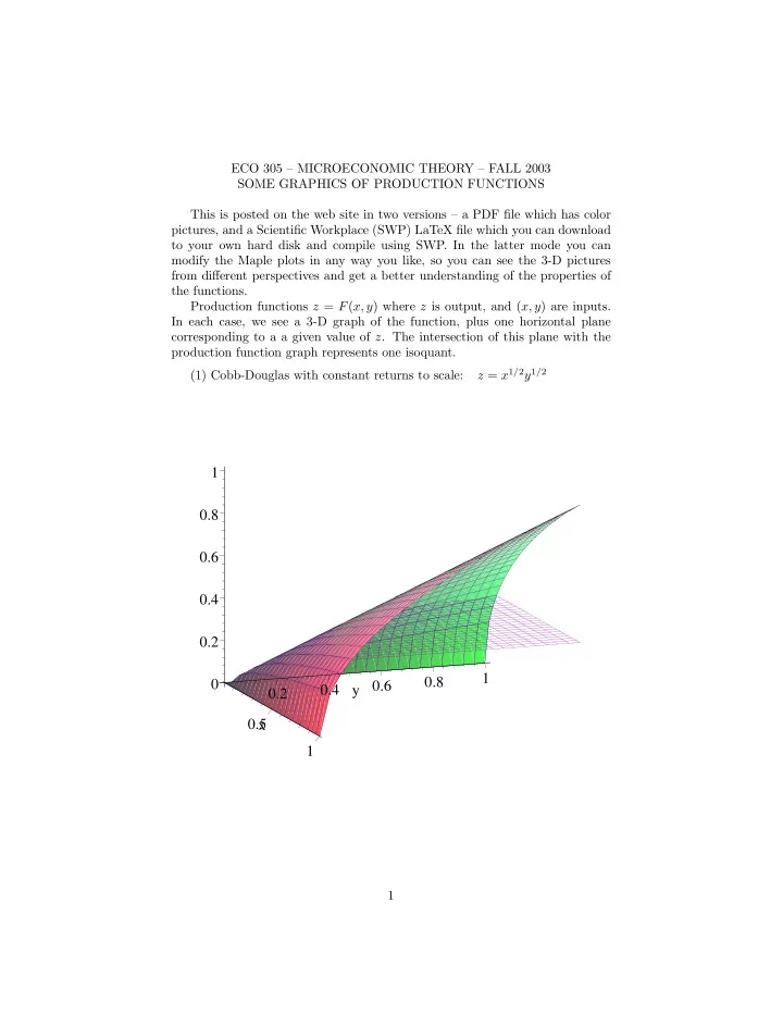
ECO 305 — MICROECONOMIC THEORY — FALL 2003 SOME GRAPHICS OF PRODUCTION FUNCTIONS This is posted on the web site in two versions — a PDF file which has color pictures, and a Scientific Workplace (SWP) LaTeX file which you can download to your own hard disk and compile using SWP. In the latter mode you can modify the Maple plots in any way you like, so you can see the 3-D pictures from different perspectives and get a better understanding of the properties of the functions. Production functions z = F(x, y) where z is output, and (x, y) are inputs. In each case, we see a 3-D graph of the function, plus one horizontal plane corresponding to a a given value of z. The intersection of this plane with the production function graph represents one isoquant. (1) Cobb-Douglas with constant returns to scale: z = x1/2y1/2
0.2 0.4 0.6 0.8 1 0.2 0.4 0.6 0.8 1 y 0.5 1 x
1
SLIDE 2
(2) Cobb-Douglas with diminishing returns to scale: z = x1/3y1/3 Note that its isoquants are indistinguishable in shape from those of the constant-returns case above, because one is a monotone increasing function of the other.
0.2 0.4 0.6 0.8 1 0.2 0.4 0.6 0.8 1 y 0.5 1 x
(3) Cobb-Douglas with increasing returns to scale: z = x3/4y3/4 Again, the isoquants are indistinguishable in shape from those of the con- stant or diminishing returns cases above. And increasing returns to scale are compatible with diminishing returns to each factor.
0.2 0.4 0.6 0.8 1 0.2 0.4 0.6 0.8 1 y 0.2 0.4 0.6 0.8 1 x
2
SLIDE 3
(4) Constant returns to scale, constant (actually = 4) elasticity of substitu- tion greater than 1: z = (x3/4 + y3/4)4/3 Two views are shown: 1 2 0.4 0.6 0.8 1 y 0.6 0.8 1 x 0.5 1 1.5 2 2.5 0.2 0.4 0.6 0.8 1 y 1 x Note z can be > 0 with one of x, y equal to 0. For example, with y = 0,we get z = x. Substitution is easy, and neither input is essential. Isoquants are very flat. 3
SLIDE 4
(5) z = (x1/2 + y1/2)2 Elasticity of substitution = 2. Still neither input is essential, but substitution is a little less easy than before; isoquants are a little more curved.
1 2 3 4 0.2 0.4 0.6 0.8 1 y 0.4 0.6 0.8 1 x
4
SLIDE 5 (6) Elasticity of substitution less than 1: Note that the isoquants are asymptotic not to the axes, but to positive values of x and y. For example, the isoquant z = 0.2 is asymptotic to the lines x = 0.2 and y = 0.2. In other words, we need a certain minimum quantity of each input to produce a desired output
- level. Unless you have x > 0.2, no amount of y will give output z = 0.2. Input
substitution is limited, and both inputs are essential. z = (x−1 + y−1)−1, σ = 0.5
0.1 0.2 0.3 0.4 0.5 0.2 0.4 0.6 0.8 1 y 1 x
z = (x−4 + y−4)−1/4, σ = 0.2
0.2 0.4 0.6 0.8 0.2 0.4 0.6 0.8 1 y 0.5 1 x
5