02110 String indexing Computational geometry Introduction to - - PowerPoint PPT Presentation

02110

Inge Li Gørtz

• Balanced binary search trees: Red-black trees and 2-3-4 trees
• Amortized analysis
• Dynamic programming
• Network flows
• String matching
• String indexing
• Computational geometry
• Introduction to NP-completeness
• Randomized algorithms

Overview

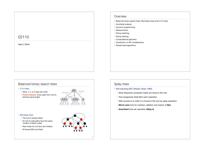
• 2-3-4 trees.
• Allow 1, 2, or 3 keys per node
• Perfect balance. Every path from root to

leaf has same length.

• Red-black trees.
• The root is always black
• All root-to-leaf paths have the same

number of black nodes.

• Red nodes do not have red children
• All leaves (NIL) are black

Balanced binary search trees

3

R H N C A

E I A S

A A C H I N E R S

smaller than E between E and R larger than R

• Self-adjusting BST (Sleator-Tarjan 1983).
• Most frequently accessed nodes are close to the root.
• Tree reorganizes itself after each operation.
• After access to a node it is moved to the root by splay operation.
• Worst case time for insertion, deletion and search is O(n).
• Amortized time per operation O(log n).

Splay trees

• Splay(x): do following rotations until x is the root. Let y be the parent of x.
• right (or left): if x has no grandparent.

Splaying

right rotation at x (and left rotation at y)

x y

a b c a b c

y x

right left

• Splay(x): do following rotations until x is the root. Let p(x) be the parent of x.
• right (or left): if x has no grandparent.
• zig-zag (or zag-zig): if one of x,p(x) is a left child and the other is a right

child.

Splaying

zig-zag at x

x x x w w w z z z

a b c d a a b b c c d d

• Splay(x): do following rotations until x is the root. Let y be the parent of x.
• right (or left): if x has no grandparent.
• zig-zag (or zag-zig): if one of x,y is a left child and the other is a right child.
• roller-coaster: if x and p(x) are either both left children or both right

children.

Splaying

right roller-coaster at x (and left roller-coaster at z)

x x x y y y z z z

a a a b b b c c c d d d

Dynamic set implementations

Worst case running times (except splay trees)

8

Implementation search insert delete minimum maximum successor predecessor linked lists O(n) O(1) O(1) O(n) O(n) O(n) O(n)

• rdered array

O(log n) O(n) O(n) O(1) O(1) O(log n) O(log n) BST O(h) O(h) O(h) O(h) O(h) O(h) O(h) 2-3-4 tree O(log n) O(log n) O(log n) O(log n) O(log n) O(log n) O(log n) red-black tree O(log n) O(log n) O(log n) O(log n) O(log n) O(log n) O(log n) splay tree O(log n)† O(log n)† O(log n)† O(log n)† O(log n)† O(log n)† O(log n)† †: amortized running time

Amortized analysis

• Amortized analysis.
• Time required to perform a sequence of data operations is averaged over all the operations

performed.

• Example: dynamic tables with doubling and halving
• If the table is full copy the elements to a new array of double size.
• If the table is a quarter full copy the elements to a new array of half the size.
• Worst case time for insertion or deletion: O(n)
• Amortized time for insertion and deletion: O(1)
• Any sequence of n insertions and deletions takes time O(n).
• Methods.
• Aggregate method
• Accounting method
• Potential method
• General algorithmic technique
• Can be used when the problem have “optimal substructure”:

solution can be constructed from optimal solutions to subproblems.

• Examples
• Weighted interval scheduling
• Segmented least squares
• Sequence alignment
• Shortest paths (Bellman-Ford)

Dynamic Programming Sequence alignment

A C A A G T C C A T G T A C G T A 1 2 2 C 1 2 3 G 2 2 1 T 2 3 1 Penalty matrix SA(Xi, Yj) =                jδ if i = 0 iδ if j = 0 min      α(xi, yj) + SA(Xi−1, Yj−1), δ + SA(Xi, Yj−1), δ + SA(Xi−1, Yj)}

• therwise

δ = 1 SA(X5, Y3) Depends on ?

11

Sequence alignment: Finding the solution

A C A A G T C 1 2 3 4 5 6 7 C 1 1 1 2 3 4 5 6 A 2 1 2 1 2 3 4 5 T 3 2 3 2 3 3 3 4 G 4 3 4 3 4 3 4 5 T 5 4 5 4 5 4 3 4 A C G T A 1 2 2 C 1 2 3 G 2 2 1 T 2 3 1 Penalty matrix

SA(Xi, Yj) =                jδ if i = 0 iδ if j = 0 min      α(xi, yj) + SA(Xi−1, Yj−1), δ + SA(Xi, Yj−1), δ + SA(Xi−1, Yj)}

• therwise

δ = 1 A C A A G T C

← ← ← ← ← ← ←

C ↑

↖ ↖ ← ← ← ← ↖

A ↑

↖ ↖ ↖ ↖ ← ← ←

T

↑ ↑ ↑ ↑ ↖ ↖ ↖ ←

G

↑ ↑ ↖ ↑ ↖ ↖ ↖ ↖

T

↑ ↑ ↑ ↑ ↖ ↑ ↖ ←

12

Bellman-Ford

OPT(i, v) = { if i = 0 min{OPT(i − 1,v), min(v,w)∈E{OPT(i − 1,w) + cvw}}

• therwise

Bellmann-Ford(G,s,t) for each node v ∈ V M[0,v] = ∞ M[0,t] = 0. for i=1 to n-1 for each node v ∈ V M[i,v] = M[i-1,v] for each edge (v,w) ∈ E M[i,v] = min(M[i,v], M[i-1,w] + cvw

13

Example

s t 9 10 6 18 15

• 8

30 20 44

• 16

11 6 19 6 16 ∞ ∞ ∞ ∞ ∞ ∞ ∞

Bellmann-Ford(G,s,t) for each node v ∈ V M[0,v] = ∞ M[0,t] = 0. for i=1 to n-1 for each node v ∈ V M[i,v] = M[i-1,v] for each edge (v,w) ∈ E M[i,v] = min(M[i,v], M[i-1,w] + cvw

14

1 2 3 4 5 6 7 s ∞ a ∞ b ∞ c ∞ d ∞ e ∞ f ∞ t

a d b e c f

Example

s t 9 10 6 18 15

• 8

30 20 44

• 16

11 6 19 6 16

Bellmann-Ford(G,s,t) for each node v ∈ V M[0,v] = ∞ M[0,t] = 0. for i=1 to n-1 for each node v ∈ V M[i,v] = M[i-1,v] for each edge (v,w) ∈ E M[i,v] = min(M[i,v], M[i-1,w] + cvw

15

a d b e c f

1 2 3 4 5 6 7 s ∞ a ∞ b ∞ c ∞ d ∞ e ∞ f ∞ t ∞ ∞ ∞ 44 16 6 19

Example

s t 9 10 6 18 15

• 8

30 20 44

• 16

11 6 19 6 16 ∞ ∞ ∞ 19 6 44 16 59 29 36

Bellmann-Ford(G,s,t) for each node v ∈ V M[0,v] = ∞ M[0,t] = 0. for i=1 to n-1 for each node v ∈ V M[i,v] = M[i-1,v] for each edge (v,w) ∈ E M[i,v] = min(M[i,v], M[i-1,w] + cvw)

16

a d b e c f

1 2 3 4 5 6 7 s ∞ ∞ a ∞ ∞ b ∞ ∞ c ∞ 44 d ∞ 16 e ∞ 6 f ∞ 19 t 59 29 36 44 16 6

Network Flow

• Network flow:
• graph G=(V,E).
• Special vertices s (source) and t (sink).
• Every edge (u,v) has a capacity c(u,v) ≥ 0.
• Flow:
• capacity constraint: every edge e has a flow 0 ≤ f(u,v) ≤ c(u,v).
• flow conservation: for all u ≠ s, t: flow into u equals flow out of u.
• Value of flow f is the sum of flows out of s minus sum of flows into s:
• Maximum flow problem: find s-t flow of maximum value

1 2 2 2 2 1 2 2 1 s t

X

v:(v,u)∈E

f(v, u) = X

v:(u,v)∈E

f(u, v)

u

|f| = X

v:(s,v)∈E

f(s, v) − X

v:(v,s)∈E

f(v, s)

Network flow: s-t Cuts

• Cut: Partition of vertices into S and T, such that s ∈ S and t ∈ T.
• Capacity of cut: total capacity of edges going from S to T.
• Flow across cut: flow from S to T minus flow from T to S.
• Value of flow any flow |f| ≤ c(S,T) for any s-t cut (S,T).
• Suppose we have found flow f and cut (S,T) such that |f| = c(S,T). Then f is a

maximum flow and (S,T) is a minimum cut.

s t S T

• Augmenting path (definition different than in CLRS): s-t path where
• forward edges have leftover capacity
• backwards edges have positive flow
• There is no augmenting path <=> f is a maximum flow.
• Ford-Fulkerson algorithm:
• Repeatedly find augmenting path, use it, until no augmenting path exists
• Running time: O(|f*| m).
• Edmonds-Karp algorithm:
• Repeatedly find shortest augmenting path, use it, until no augmenting path exists
• Use BFS to find a shortest augmenting path.
• Running time: O(nm2)
• Find minimum cut. All vertices to which there is an augmenting path from s goes into

S, rest into T.

Augmenting paths

s t

f1 < c1 f2 > 0 f3 < c3 f4 < c4 f5 > 0 f6 > 0 +δ +δ +δ

• δ
• δ
• δ
• Scaling parameter Δ
• Only consider edges with capacity at least Δ in residual graph Gf(Δ).
• Example: Δ = 4

Scaling algorithm

Gf(4) Gf

s

1 1 1 4 4 1 3 4 2 2 2 6

t

3 3 3 3 5 4 4 4

s

1 1 1 4 4 1 3 4 2 2 2 6

t

3 3 3 3 5 4 4 4

20

• Can model and solve many problems via maximum flow.
• Maximum bipartite matching
• k edge-disjoint paths
• capacities on vertices
• Many sources/sinks
• lower bounds on flow on edges.
• assignment problems: Example. X doctors, Y holidays, each doctor should work

at at most c holidays, each doctor is available at some of the holidays.

Network flow

s t

1 1 c c c

• String matching problem:
• string T (text) and string P (pattern) over an alphabet Σ. |T| = n, |P| = m.
• Report all starting positions of occurrences of P in T.
• String matching automaton. Running time: O(n + m|Σ|)
• Knuth-Morris-Pratt (KMP). Running time: O(m + n)

String Matching

Finite Automaton

• Finite automaton: alphabet Σ = {a,b,c}. P= ababaca.

a b a b a c a a a a b a b

starting state accepting state

Finite Automaton

• Finite automaton: alphabet Σ = {a,b,c}. P= ababaca.

a b a b a c a a a a b a b

starting state accepting state longest prefix of P that is a suffix of ‘abaa'

Finite Automaton

• Finite automaton: alphabet Σ = {a,b,c}. P = ababaca.

a b a b a c a a a a b a b b a c b a b a b a b a b a c a b T =

Knuth-Morris-Pratt (KMP)

• Matched P[1…q]: Find longest block P[1..k] that matches end of P[2..q].
• Find longest prefix P[1...k] of P that is a proper suffix of P[1...q]
• Array π[1…m]:
• π[q] = max k < q such that P[1...k] is a suffix of P[1…q].
• Can be seen as finite automaton with failure links:

a a a b a a a a b a b a a a a b a b a

i 1 2 3 4 5 6 7 π[i] 1 2 3 1

a b a b a c a

1 2 3 4 5 6

KMP matching

• KMP: Can be seen as finite automaton with failure links:
• longest prefix of P that is a suffix of what we have matched until now.

b a c b a b a b a b a b a c a b T = a b a b a c a

1 2 3 4 5 6

String Indexing

• String indexing problem. Given a string S of characters from an alphabet Σ.

Preprocess S into a data structure to support

• Search(P): Return starting position of all occurrences of P in S.
• Tries.
• Compact trie. Chains of nodes with a single child merged into a single node
• Suffix tree. Compact trie over all the suffixes of a string.

b y

S2 S1

s s s

S4 S6 S3

e e e e a a l l l l h h t

S5

$ $ $ $ $ $

S7

$

String Indexing

• String indexing problem. Given a string S of characters from an alphabet Σ.

Preprocess S into a data structure to support

• Search(P): Return starting position of all occurrences of P in S.
• Tries.
• Compact trie. Chains of nodes with a single child merged into a single node
• Suffix tree. Compact trie over all the suffixes of a string.

b y $ S2 s e a $ S4 l ls $ S1 he l l s $ S6 S3 S5 S7 $ t e a $ h e $

• Suffix tree. Compact trie over all suffixes of a string.
• Suffix trees can be used to solve the String indexing

problem in:

• Space: O(n)
• Search time: O(m+occ)
• Preprocessing: O(sort(n,|Σ|)) time

Suffix tree

$

b

1

a n a a n a

$ 6

n a

$ 4

n a

$ 2

na n a

$ 3 5 $ $ 7

• Suffix tree. Compact trie over all suffixes of a string.
• Suffix trees can be used to solve the String indexing

problem in:

• Space: O(n)
• Search time: O(m+occ)
• Preprocessing: O(sort(n,|Σ|)) time

Suffix tree

0 1 2 3 4 5 6 b a n a n a $

1

[2,2]

6 4 2 3 5 7

[3,4] [7,7] [5,7] [7,7] [7,7] [7,7] [1,7] [3,4] [5,7]

Longest common substring

pie is the longest common substring

$1 9 18 15 12 7 16 3 6 14 11 2 10 13 5 1 17 8 4 $2 $1 $1 $1 $2 $2 $2 $2 $2 p p p p p i i i e e e e e e e e s s s s s s i i i s s $1 $2 $2 $2 s s e e . . . . . . . . . . . . . . . e e $2 $2 $2 $2 $1 $2 . . . e $2 s p s i e $1 $2 . . . p s i $1 $2 e . . . p s i $1 $2 e . . .

Example: Find longest common substring of piespies and piepiees:

• Median/Select.
• Quick-sort
• Closest pair

Randomized algorithms

• Use hashtable to store which square a point is in. Only store points already

looked at (red points).

Closest Pair of Points: Randomized algorithm

3 4 11 9 10 15 5 1 2 14 12 6 13 8 7 δ2 δ1

• Reduction. Problem X polynomial reduces to problem Y if arbitrary instances of

problem X can be solved using:

• Polynomial number of standard computational steps, plus
• Polynomial number of calls to oracle that solves problem Y.
• Notation. X ≤P Y.
• We pay for time to write down instances sent to black box ⇒ instances of Y must

be of polynomial size.

Polynomial-time reduction

35

• Purpose. Classify problems according to relative difficulty.
• Design algorithms. If X ≤P Y and Y can be solved in polynomial-time, then

X can also be solved in polynomial time.

• Establish intractability. If X ≤P Y and X cannot be solved in polynomial-time,

then Y cannot be solved in polynomial time.

• Establish equivalence. If X ≤P Y and Y ≤P X, we use notation X =P Y.

Polynomial-time reductions

up to a polynomial factor

36

• P solvable in deterministic polynomial time.
• NP solvable in non-deterministic polynomial time/ has an efficient (polynomial time)

certifier.

• P⊆NP (every problem T which is in P is also in NP).
• It is not known (but strongly believed) whether the inclusion is proper, that is whether

there is a problem in NP which is not in P .

• There is subclass of NP which contains the hardest problems, NP-complete

problems:

• X is NP-Complete if
• X ∈ NP
• Y ≤P X for all Y ∈ NP

P vs NP

37

• 1. Prove X ∈ NP (that it can be verified in polynomial time).
• 2. Select a known NP-complete problem Y.
• 3. Give a polynomial time reduction from Y to X:
• Explain how to turn an instance of Y into one or more instances of X
• Explain how to use a polynomial number of calls to the black box algorithm/
• racle for X to solve Y.
• Prove/argue that the reduction is correct.

How to prove a problem is NP-complete

38

• 02282 Algorithms for massive data sets
• 02249 Computationally Hard Problems
• 01227 Graph theory
• 02807 Computational Tools for Data Science
• Thesis

How to study algorithms at DTU

Thank you