INF3130: Dynamic Programming 12 sept. 2019 In the textbook: Ch. 9, - PowerPoint PPT Presentation

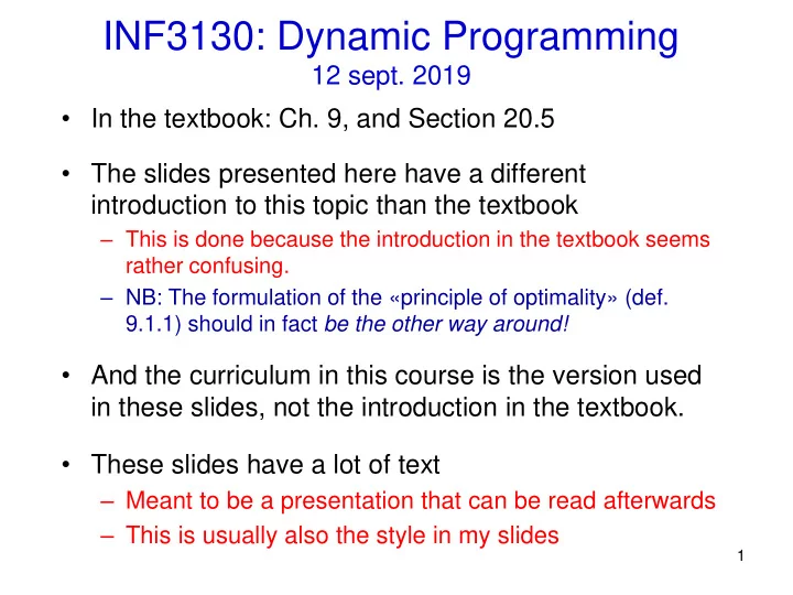
INF3130: Dynamic Programming 12 sept. 2019 • In the textbook: Ch. 9, and Section 20.5 • The slides presented here have a different introduction to this topic than the textbook – This is done because the introduction in the textbook seems rather confusing. – NB: The formulation of the «principle of optimality» (def. 9.1.1) should in fact be the other way around! • And the curriculum in this course is the version used in these slides, not the introduction in the textbook. • These slides have a lot of text – Meant to be a presentation that can be read afterwards – This is usually also the style in my slides 1

Dynamic programming Dynamic programming was formalised by Richard Bellmann (RAND Corporation) in the 1950’es. – «programming» should here be understood as planning, or making decisions. It has nothing to do with writing code. – ” Dynamic ” should indicate that it is a stepwise process. But was that the real background for the name?? 2

A simple example We are given a matrix W with positive «weights» in each cell : W: Problem : Find the «best» path (lowest sum of weights) from upper left to lower right corner. 12 5 35 7 21 NB: The shown red path is radomly chosen, and is 4 29 8 19 14 probably not the best path (has weight = 255) 8 3 19 20 24 37 84 78 15 62 We use a new matrix P to store intermediate results: 26 13 40 33 12 P[i,j] = The weight of the best path from the start (upper left) to cell [i,j]. 21 60 27 18 17 The «recurrence relation» will be: P (initialization in black) P[i, j] = min(P[i-1, j], P[i, j-1]) + W[i,j ] • We can initialialize by filling in the leftmost column and 12 17 52 59 80 topmost row, as shown to the left. 16 45 53 72 86 • We can the fill in P according to the formula above 24 27 46 66 90 111 124 81 143 61 Questions (exercises for next week): 87 100 140 114 126 - In which order should P be filled out? 108 160 167 132 143 - How can we find the shortest path itself? 3 - What is the complexity of this algorithm?

Another problem (Ch. 9.4) Find the «Longest Common Subsequence» of two strings: P (pattern) and T (text) 7 5 1 2 3 4 6 T e f h k p p g P g e h p f p 1 2 3 4 5 6 The Longest Common Subsequence is here «e, h, p, p» «Length of Longest Commom Subsequence» (LCS) is 4. 4

An idea for finding LCS We will use an interger matrix L[0:m, 0:n] as shown below, where we imagine that the string P = P[1:m] is placed downwords along the left side of L, and T = T[1:n] is placed above D from left to right (at corresponding indices). ( NB: This is a slightly different use of indices than in Sectons 9.4 and 20.5). Our plan is then to systematically fill in this table so that L[i, j] = LSC( P[1:i], T[1:j] ) We will do this from «smaller» to «larger» index pairs (i, j), by taking column after column from left to right (but row after row from top to bottom would also work). The value we are looking for, LSC(P, T), will then occur in L[m, n] when all entries are filled. T … 0 1 j -1 j n 0 P 1 The matrix L: ... i -1 i ? 5 m

Example: P = «gehpfp» and T = «efhkppg» We initialize the leftmost column and the topmost row as below - Why is it correct with zeroes here? - Note that these celles correspond to the empty prefix of P and/or the empty prefix of T. T e f h k p p g L j 0 1 2 3 4 5 6 7 0 0 0 0 0 0 0 0 0 We have filled in g 1 0 0 0 0 0 0 0 1 a few more e 2 0 1 1 1 entries of L by intuition h 0 1 1 2 3 P p 0 1 4 f 5 0 We hope to get p 0 4? 6 4 here! 6 i

The general formula for filling L T e f h k p p g We want to find: L[i,j] L 0 1 2 3 4 5 6 7 and assume we have 0 0 0 0 0 0 0 0 0 already computed: g 0 0 0 0 0 0 0 1 1 e 2 0 1 1 1 L[i-1,j-1] L[i-1,j] h 0 1 1 2 3 P L[i,j-1] (Find: L[i,j]) p 0 1 4 f 5 0 p 0 4? 6 Case 1: Case 2: If Pi ≠ Tj then If Pi = Tj then L[i,j] = L[i-1,j-1] +1 L[i,j] = max( L[i,j-1], L[i-1,j] ) WHY? WHY? 7

Case 1: If Pi = Tj then L[i-1,j-1] L[i-1,j] L[i,j] = L[i-1,j-1] +1 L[i,j-1] (Find: L[i,j]) Case 2: If Pi ≠ Tj then L[i,j] = max( L[i,j-1], L[i-1,j] ) T[1:j-1] T[1:j-1] T[j] P[1:i-1] P[1:i-1] T[1:j-1] T[1:j-1] T[j] P[1:i-1] P[1:i-1] 8 P[i] P[i]

Using the formula for filling L T e f h k p p g L 0 1 2 3 4 5 6 7 We want to find: L[i,j] and assume we have 0 0 0 0 0 0 0 0 0 already computed: g 0 0 0 0 0 0 0 1 1 L[i-1,j-1] L[i-1,j] e 2 0 1 1 1 1 1 1 1 h 0 1 1 2 2 2 2 2 3 L[i,j-1] (Find: L[i,j]) P p 0 1 1 2 2 3 3 3 4 f 5 0 1 2 2 2 3 3 3 4 p 0 1 2 2 2 3 4 6 Hurrah! Case 1: Case 2: If Pi ≠ Tj then If Pi = Tj then L[i,j] = max( L[i,j-1], L[i-1,j] ) L[i,j] = L[i-1,j-1] +1 9

Finding the Longest Common Subsequence itself e f h k p p g T L 0 1 2 3 4 5 6 7 Case 1 0 0 0 0 0 0 0 0 0 If Pi = Tj then L[i,j] = L[i-1,j-1] +1 0 g 1 0 0 0 0 0 0 1 Case 2 1 1 e 0 1 1 1 1 1 2 If Pi ≠ Tj then h 0 1 1 2 2 2 2 2 3 P L[i,j] = max( L[i,j-1], L[i-1,j] ) 3 p 4 0 1 1 2 2 3 3 3 u 0 1 1 2 2 3 3 5 4 0 4 p 6 1 2 2 2 3 2. The red arrows indicate 1. To find the actual Longest Common the letters included in the Subsequence we highlight entries, Longest Common backwards from lower right, what Subsequence «caused» each value (green numbers) 10

We’ll now look at the problem discussed in Chapter 20.5: «Approximate String Matching»: Given: A long string T and a shorter string P Problem: Find strings «similar» to P in T P: u t t x v T: b s u t t v r t o x i g u t t v x l b t s k u t t z x v k l v h u u t t x v n x u t z t x v w Questions: - What do we mean by a «similar string»? - Can we quantify the degree of simularity? We’ll first look at how to define and find: The Edit Distance between P and T 11

The «edit distance» between two strings We observe that any string P can be converted to another string T by some sequence of the following opertions (usally by many different such sequences): Substitution: One symbol in P is changed to another symbol. Addition: A new symbol is inserted somwhere in P . Removing: One symbol is removed from P . The «Edit Distance» , ED ( P , T ), between two strings P and T is: The smallest number of such operations needed to convert P to T (or T to P! Note that the definition is symmetric in P and T!) Example. logarithm  alogarithm  algarithm  algorithm (Steps: +a, -o, a->o) P T 12 Thus ED(” logarithm ”, ” algorithm ”) = 3 (as there are no shorter ways!)

To find ED(P,T) we use a similar setup as for LCS We use an interger matrix D[0:m, 0:n], where P = P[1:m] is placed downwords along the left side of D, and T = T[1:n] is placed above D Our plan is again to systematically fill in this table, but so that D[i, j] = Edit Distance between the strings P[1:i] and T[1:j] Like before we will do this e.g. by taking column after column from left to right. The value we are looking for, ED(P, T), will then occur in D[m, n] when all entries are filled in. T … 0 1 j -1 j n 0 1 The matrix D : ... P i -1 i ? 13 m

Example: P = «anne» and T = «ane» - We initialize the leftmost column and the topmost row as below - Why is this correct? - Note that these celles correspond to the empty prefix of P and/or the empty prefix of T. T a n e D j 0 1 2 3 0 1 2 3 0 a 1 1 n 2 2 P n 3 3 e 4 4 14 i

More of P = «anne» and T = «ane» We’ll look a general cell D[i,j], and try to find how the value here can be computed from the values in the tree cells over and to the left. We first assume that P[i]= T[j](as below). We know that P[1: i-1] can be converted to T[1:j-1] in D[i-1, j-1] steps, and thus «T[1:j- 1]‘n’» can also be transformed into «D[i-1, j-1 ] ‘n’» in D[i-1, j-1] steps. a n e T D 0 1 2 3 j P 0 1 2 3 0 Thus : a 1 1 if P[i] = T[j], then n 2 D[i-1,j-1] D[i-1, j] . 2 D[i,j] = D[i-1, j-1] n 3 3 D[i, j-1]. D[i, j] . e 4 . . 4 15 i

L[i-1,j-1] L[i-1,j] Case 1: If Pi = Tj then L[i,j-1] (Find: L[i,j]) D[i,j] = D[i-1, j-1] T[1:j-1] T[1:j-1] T[j] P[1:i-1] P[1:i-1] T[1:j-1] T[1:j-1] T[j] Equal P[1:i-1] P[1:i-1] 16 P[i] P[i]

More of P = «anne» and T = «ane» We again look a general cell D[i,j], but we now assume that P[i] ≠ T[j] . We know that: P[1: i-1] can be transformed to T[1: j-1] in D[i-1, j-1] steps, and we can thus transform «T[1: j- 1]‘x’» to « P[1: j-1 ]‘y’» in D[i-1, j-1] +1 steps. Likewise we get: a x e T We can transform «T[1: j-1]» into «P[1: i- 1]‘y’» in D[i, j -1] +1 steps. D 0 1 2 3 j «T[1: j-1]» into «P[1: i-1 ] ‘y’» in P 0 1 2 3 D[i-1, j] +1 steps. 0 a 1 1 Thus we can do the transformation from n 2 2 D[i-1,j-1] D[i-1, j] . «T[1: j- 1]‘x’» into «P[1: i- 1] ‘y’» in the minimum number of y 3 D[i, j-1] D[i, j] . 3 steps used in these three e 4 . . 4 scenarios. We therefore obtain the formula on next page. 17 i

L[i-1,j-1] L[i-1,j] Case 2: L[i,j-1] (Find: L[i,j]) If Pi ≠ Tj then D[i,j] = min( D[i-1,j-1], D[i,j-1], D[i-1,j] ) + 1 T[1:j-1] T[1:j-1] T[j] P[1:i-1] P[1:i-1] T[1:j-1] T[1:j-1] T[j] Different P[1:i-1] P[1:i-1] 18 P[i] P[i]