[PPT] - 00110010010101101001100111010110 ...adbck7d... Observer PowerPoint Presentation

SLIDE 1

SFI CSSS, Beijing China, July 2006: Information Theory, Part II 1

Information Theory: Part II Applications to Stochastic Processes

We now consider applying information theory to a long sequence of

measurements.

· · · 00110010010101101001100111010110 · · ·

In so doing, we will be led to two important quantities
1. Entropy Rate: The irreducible randomness of the system.
2. Excess Entropy: A measure of the complexity of the sequence.

Context: Consider a long sequence of discrete random variables. These could be:

1. A long time series of measurements
2. A symbolic dynamical system
3. A one-dimensional statistical mechanical system

c

David P

. Feldman and SFI

http://hornacek.coa.edu/dave

SFI CSSS, Beijing China, July 2006: Information Theory, Part II 2

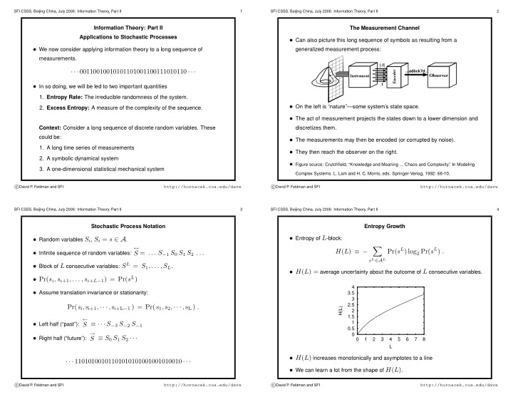
The Measurement Channel

Can also picture this long sequence of symbols as resulting from a

generalized measurement process:

Instrument 1 |A| Encoder ...adbck7d...

Observer

On the left is “nature”—some system’s state space.
The act of measurement projects the states down to a lower dimension and

discretizes them.

The measurements may then be encoded (or corrupted by noise).
They then reach the observer on the right.
Figure source: Crutchfield, “Knowledge and Meaning ... Chaos and Complexity.” In Modeling

Complex Systems. L. Lam and H. C. Morris, eds. Springer-Verlag, 1992: 66-10.

c

David P

. Feldman and SFI

http://hornacek.coa.edu/dave

SFI CSSS, Beijing China, July 2006: Information Theory, Part II 3

Stochastic Process Notation

Random variables Si, Si = s ∈ A.
Infinite sequence of random variables:

↔

S = . . . S−1 S0 S1 S2 . . .

Block of L consecutive variables: SL = S1, . . . , SL.
Pr(si, si+1, . . . , si+L−1) = Pr(sL)
Assume translation invariance or stationarity:

Pr( si, si+1, · · · , si+L−1 ) = Pr( s1, s2, · · · , sL ) .

Left half (“past”):

←

S ≡ · · · S−3 S−2 S−1

Right half (“future”):

→

S ≡ S0 S1 S2 · · · · · · 11010100101101010101001001010010 · · ·

c

David P

. Feldman and SFI

http://hornacek.coa.edu/dave

SFI CSSS, Beijing China, July 2006: Information Theory, Part II 4

Entropy Growth

Entropy of L-block:

H(L) ≡ −

sL∈AL

Pr(sL) log2 Pr(sL) .

H(L) = average uncertainty about the outcome of L consecutive variables.

0.5 1 1.5 2 2.5 3 3.5 4 1 2 3 4 5 6 7 8 H(L) L

H(L) increases monotonically and asymptotes to a line
We can learn a lot from the shape of H(L).

c

David P

. Feldman and SFI

http://hornacek.coa.edu/dave

SLIDE 2

SFI CSSS, Beijing China, July 2006: Information Theory, Part II 5

Entropy Rate

Let’s first look at the slope of the line:

L H(L)

µ

+ h L E

E H(L)

Slope of H(L): hµ(L) ≡ H(L) − H(L−1)
Slope of the line to which H(L) asymptotes is known as the entropy rate:

hµ = lim

L→∞ hµ(L).

c

David P

. Feldman and SFI

http://hornacek.coa.edu/dave

SFI CSSS, Beijing China, July 2006: Information Theory, Part II 6

Entropy Rate, continued

Slope of the line to which H(L) asymptotes is known as the entropy rate:

hµ = lim

L→∞ hµ(L).

hµ(L) = H[SL|S1S1 . . . SL−1]
I.e., hµ(L) is the average uncertainty of the next symbol, given that the

previous L symbols have been observed.

c

David P

. Feldman and SFI

http://hornacek.coa.edu/dave

SFI CSSS, Beijing China, July 2006: Information Theory, Part II 7

Interpretations of Entropy Rate

Uncertainty per symbol.
Irreducible randomness: the randomness that persists even after accounting

for correlations over arbitrarily large blocks of variables.

The randomness that cannot be “explained away”.
Entropy rate is also known as the Entropy Density or the Metric Entropy.
hµ = Lyapunov exponent for many classes of 1D maps.
The entropy rate may also be written: hµ = limL→∞

H(L) L

.

hµ is equivalent to thermodynamic entropy.
These limits exist for all stationary processes.

c

David P

. Feldman and SFI

http://hornacek.coa.edu/dave

SFI CSSS, Beijing China, July 2006: Information Theory, Part II 8

How does hµ(L) approach hµ?

For finite L , hµ(L) ≥ hµ. Thus, the system appears more random than it is.

1 L h (L)

µ

hµ E H(1)

We can learn about the complexity of the system by looking at how the

entropy density converges to hµ.

c

David P

. Feldman and SFI

http://hornacek.coa.edu/dave

SLIDE 3

SFI CSSS, Beijing China, July 2006: Information Theory, Part II 9

The Excess Entropy 1 L h (L)

µ

hµ E H(1)

The excess entropy captures the nature of the convergence and is defined

as the shaded area above:

E ≡

∞

L=1

[hµ(L) − hµ] .

E is thus the total amount of randomness that is “explained away” by

considering larger blocks of variables.

c

David P

. Feldman and SFI

http://hornacek.coa.edu/dave

SFI CSSS, Beijing China, July 2006: Information Theory, Part II 10

Excess Entropy: Other expressions and interpretations Mutual information

One can show that E is equal to the mutual information between the “past”

and the “future”:

E = I(

←

S;

→

S) ≡

{

↔

s }

Pr(

↔

s ) log2

Pr(

↔

s ) Pr(

←

s )Pr(

→

s )

.
E is thus the amount one half “remembers” about the other, the reduction in

uncertainty about the future given knowledge of the past.

Equivalently, E is the “cost of amnesia:” how much more random the future

appears if all historical information is suddenly lost.

c

David P

. Feldman and SFI

http://hornacek.coa.edu/dave

SFI CSSS, Beijing China, July 2006: Information Theory, Part II 11

Excess Entropy: Other expressions and interpretations Geometric View

E is the y-intercept of the straight line to which H(L) asymptotes.
E = limL→∞ [H(L) − hµL] .

L H(L)

µ

+ h L E

E H(L)

c

David P

. Feldman and SFI

http://hornacek.coa.edu/dave

SFI CSSS, Beijing China, July 2006: Information Theory, Part II 12

Excess Entropy Summary

Is a structural property of the system — measures a feature complementary

to entropy.

Measures memory or spatial structure.
Lower bound for statistical complexity, minimum amount of information

needed for minimal stochastic model of system

c

David P

. Feldman and SFI

http://hornacek.coa.edu/dave

SLIDE 4

SFI CSSS, Beijing China, July 2006: Information Theory, Part II 13

Example I: Fair Coin

2 4 6 8 10 12 14 16 2 4 6 8 10 12 14 H(L) L H(L): Fair Coin H(L): Biased Coin, p=.7

For fair coin, hµ = 1.
For the biased coin, hµ ≈ 0.8831.
For both coins, E = 0.
Note that two systems with different entropy rates have the same excess

entropy.

c

David P

. Feldman and SFI

http://hornacek.coa.edu/dave

SFI CSSS, Beijing China, July 2006: Information Theory, Part II 14

Example II: Periodic Sequence

0.5 1 1.5 2 2.5 3 3.5 4 4.5 2 4 6 8 10 12 14 16 18 H(L) L H(L) E + hµL 0.2 0.4 0.6 0.8 1 1.2 1.4 2 4 6 8 10 12 14 16 18 hµ(L) L hµ(L)

Sequence: . . . 1010111011101110 . . .

c

David P

. Feldman and SFI

http://hornacek.coa.edu/dave

SFI CSSS, Beijing China, July 2006: Information Theory, Part II 15

Example II, continued

Sequence: . . . 1010111011101110 . . .
hµ ≈ 0; the sequence is perfectly predictable.
E = log2 16 = 4: four bits of phase information
For any period-p sequence, hµ = 0 and E = log2 p.

For more than you probably ever wanted to know about periodic sequences, see Feldman and Crutchfield, Synchronizing to Periodicity: The Transient Information and Synchronization Time of Periodic Sequences. Advances in Complex Systems. 7(3-4): 329-355, 2004.

c

David P

. Feldman and SFI

http://hornacek.coa.edu/dave

SFI CSSS, Beijing China, July 2006: Information Theory, Part II 16

Example III: Random, Random, XOR

2 4 6 8 10 12 14 2 4 6 8 10 12 14 16 18 H(L) L H(L) E + hµL 0.2 0.4 0.6 0.8 1 1.2 2 4 6 8 10 12 14 16 18 hµ(L) L hµ(L)

Sequence: two random symbols, followed by the XOR of those symbols.

c

David P

. Feldman and SFI

http://hornacek.coa.edu/dave

SLIDE 5

SFI CSSS, Beijing China, July 2006: Information Theory, Part II 17

Example III, continued

Sequence: two random symbols, followed by the XOR of those symbols.
hµ = 2

3; two-thirds of the symbols are unpredictable.

E = log2 4 = 2: two bits of phase information.
For many more examples, see Crutchfield and Feldman, Chaos, 15: 25-54,

2003.

c

David P

. Feldman and SFI

http://hornacek.coa.edu/dave

SFI CSSS, Beijing China, July 2006: Information Theory, Part II 18

Excess Entropy: Notes on Terminology All of the following terms refer to essentially the same quantity.

Excess Entropy: Crutchfield, Packard, Feldman
Stored Information: Shaw
Effective Measure Complexity: Grassberger, Lindgren, Nordahl
Reduced (R´

enyi) Information: Sz´ epfalusy, Gy¨

rgyi, Csord´

as

Complexity: Li, Arnold
Predictive Information: Nemenman, Bialek, Tishby

c

David P

. Feldman and SFI

http://hornacek.coa.edu/dave

SFI CSSS, Beijing China, July 2006: Information Theory, Part II 19

Excess Entropy: Selected References and Applications

Crutchfield and Packard, Intl. J. Theo. Phys, 21:433-466. (1982); Physica D,

7:201-223, 1983. [Dynamical systems]

Shaw, “The Dripping Faucet ..., ” Aerial Press, 1984. [A dripping faucet]
Grassberger, Intl. J. Theo. Phys, 25:907-938, 1986. [Cellular automata (CAs),

dynamical systems]

Sz´

epfalusy and Gy¨

rgyi, Phys. Rev. A, 33:2852-2855, 1986. [Dynamical systems]
Lindgren and Nordahl, Complex Systems, 2:409-440. (1988). [CAs, dynamical

systems]

Csord´

as and Sz´ epfalusy, Phys. Rev. A, 39:4767-4777. 1989. [Dynamical Systems]

Li, Complex Systems, 5:381-399, 1991.
Freund, Ebeling, and Rateitschak, Phys. Rev. E, 54:5561-5566, 1996.
Feldman and Crutchfield, SFI:98-04-026, 1998. Crutchfield and Feldman, Phys. Rev.

E 55:R1239-42. 1997. [One-dimensional Ising models]

c

David P

. Feldman and SFI

http://hornacek.coa.edu/dave

SFI CSSS, Beijing China, July 2006: Information Theory, Part II 20

Excess Entropy: Selected References and Applications, continued

Feldman and Crutchfield. Physical Review E, 67:051104. 2003. [Two-dimensional

Ising models]

Feixas, et al, Eurographics, Computer Graphics Forum, 18(3):95-106, 1999. [Image

processing]

Ebeling. Physica D, 1090:42-52. 1997. [Dynamical systems, written texts, music]
Bialek, et al, Neur. Comp., 13:2409-2463. 2001. [Long-range 1D Ising models,

machine learning]

c

David P

. Feldman and SFI

http://hornacek.coa.edu/dave

SLIDE 6

SFI CSSS, Beijing China, July 2006: Information Theory, Part II 21

Transient Information T

T ≡ ∞

L=1 [E + hµL − H(L)].

T is related to the total uncertainty experienced while synchronizing to a

process.

L H(L)

µ

+ h L E E H(L) T

The shaded area is the transient information T.
T measures how difficult it is to synchronize to a sequence.

c

David P

. Feldman and SFI

http://hornacek.coa.edu/dave

SFI CSSS, Beijing China, July 2006: Information Theory, Part II 22

Some Applications in Agent-Based Modeling Settings

1. If an agent doesn’t have sufficient memory, its environment will appear more
random. In a quantitative sense, regularities that are missed (as measured by

the excess entropy) are converted into randomness (as measured by the entropy rate).

Crutchfield and Feldman, Synchronizing to the Environment: Information

Theoretic Constraints on Agent Learning. Advances in Complex Systems.

4. 251–264. 2001.
2. The average-case difficulty for an agent to synchronize to a periodic

environment is measured by the transient information.

Feldman and Crutchfield. Synchronizing to a Periodic Signal: The

Transient Information and Synchronization Time of Periodic Sequences. Advances in Complex Systems. 7. 329–355. 2004.

c

David P

. Feldman and SFI

http://hornacek.coa.edu/dave

SFI CSSS, Beijing China, July 2006: Information Theory, Part II 23

Some Applications in Agent-Based Modeling Settings, continued

3. More generally it seems likely that the entropy and mutual information are

useful tools for quantifying (a) properties of agents: e.g., how much memory they have (b) the behavior of agents: e.g, how unpredictably they act (c) properties of the environment: e.g., how structured it is

c

David P

. Feldman and SFI

http://hornacek.coa.edu/dave

SFI CSSS, Beijing China, July 2006: Information Theory, Part II 24

Estimating Probabilities

E and hµ can be estimated empirically by observing a process.

1 1 1 ...001011101000...

1 1 1 1 1 1 1 1 1 1 1 1 Pr(s )

3

Observer System A B C Process

One simply forms histograms of occurrences of particular sequences and

uses these to estimate Pr(sL), from which E and hµ may be readily calculated. For more sophisticated and accurate ways of inferring hµ, see, e.g.,

Sch¨

urmann and Grassberger. Chaos 6:414-427. 1996.

Nemenman. http://arXiv.org/physics/0207009. 2002.

c

David P

. Feldman and SFI

http://hornacek.coa.edu/dave

SLIDE 7

SFI CSSS, Beijing China, July 2006: Information Theory, Part II 25

A look ahead

Note that the observer sees measurement symbols: 0’s and 1’s.

1 1 1 ...001011101000...

1 1 1 1 1 1 1 1 1 1 1 1 Pr(s )

3

Observer System A B C Process

It doesn’t see inside the “black box” of the system.
In particular, it doesn’t see the internal, hidden states of the system, A, B,