0 1 2 3 2 1 1 3 0 0 1 2 3 2 1 1 - - PowerPoint PPT Presentation

Enumerating partial Latin rectangles

Ra´ ul F´ alcon (U. Seville ), Rebecca J. Stones (Nankai U. )

21 May 2018

1 2 3 · · 2 · 1 · 1 3 · ·

1 2 3 · · 2 · 1 · 1 3 · ·

A partial Latin rectangle is...

1 2 3 · · 2 · 1 · 1 3 · ·

A partial Latin rectangle is... an r × s matrix, [above r = 3 and s = 5]

1 2 3 · · 2 · 1 · 1 3 · ·

A partial Latin rectangle is... an r × s matrix, [above r = 3 and s = 5] contains symbols from an n-set, [above n = 4]

1 2 3 · · 2 · 1 · 1 3 · ·

A partial Latin rectangle is... an r × s matrix, [above r = 3 and s = 5] contains symbols from an n-set, [above n = 4] Latin-ness: no repeats in each row or column,

1 2 3 · · 2 · 1 · 1 3 · ·

A partial Latin rectangle is... an r × s matrix, [above r = 3 and s = 5] contains symbols from an n-set, [above n = 4] Latin-ness: no repeats in each row or column, partial-ness: we allow empty cells,

1 2 3 · · 2 · 1 · 1 3 · ·

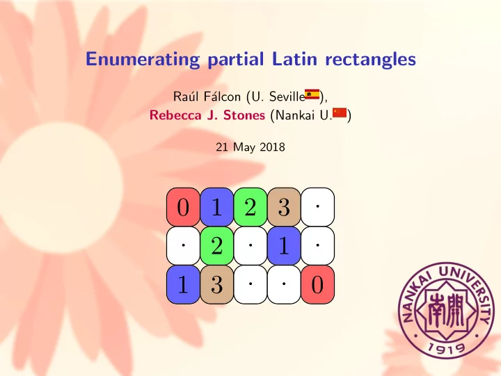
A partial Latin rectangle is... an r × s matrix, [above r = 3 and s = 5] contains symbols from an n-set, [above n = 4] Latin-ness: no repeats in each row or column, partial-ness: we allow empty cells, with m entries. [above m = 9].

1 2 3 · · 2 · 1 · 1 3 · ·

A partial Latin rectangle is... an r × s matrix, [above r = 3 and s = 5] contains symbols from an n-set, [above n = 4] Latin-ness: no repeats in each row or column, partial-ness: we allow empty cells, with m entries. [above m = 9]. This is a member of PLR(r, s, n; m) = PLR(3, 5, 4; 9).

Simple question: How many partial Latin rectangles are there?

Simple question: How many partial Latin rectangles are there? Not so easy answer (1): Latin squares are not easy to enumerate = ⇒ partial Latin rectangles are not easy to enumerate.

Simple question: How many partial Latin rectangles are there? Not so easy answer (1): Latin squares are not easy to enumerate = ⇒ partial Latin rectangles are not easy to enumerate. Not so easy answer (2): What does this even mean?

Simple question: How many partial Latin rectangles are there? Not so easy answer (1): Latin squares are not easy to enumerate = ⇒ partial Latin rectangles are not easy to enumerate. Not so easy answer (2): What does this even mean? We’ll talk about four different ways of enumerating partial Latin rectangles.

Method 1: Inclusion-Exclusion

We order the entries in m-entry partial Latin rectangles.

Method 1: Inclusion-Exclusion

We order the entries in m-entry partial Latin rectangles. We thus enumerate length-m non-clashing sequences of entries...

Method 1: Inclusion-Exclusion

We order the entries in m-entry partial Latin rectangles. We thus enumerate length-m non-clashing sequences of entries... where an entry (x, y, z) implies we put symbol z in cell (x, y).

Method 1: Inclusion-Exclusion

We order the entries in m-entry partial Latin rectangles. We thus enumerate length-m non-clashing sequences of entries... where an entry (x, y, z) implies we put symbol z in cell (x, y). The j-th entry clashes with the i-th entry when j > i and:

Method 1: Inclusion-Exclusion

We order the entries in m-entry partial Latin rectangles. We thus enumerate length-m non-clashing sequences of entries... where an entry (x, y, z) implies we put symbol z in cell (x, y). The j-th entry clashes with the i-th entry when j > i and: Blue clashes: they have same column and same symbol.

Method 1: Inclusion-Exclusion

We order the entries in m-entry partial Latin rectangles. We thus enumerate length-m non-clashing sequences of entries... where an entry (x, y, z) implies we put symbol z in cell (x, y). The j-th entry clashes with the i-th entry when j > i and: Blue clashes: they have same column and same symbol. Red clashes: they have same row and same symbol.

Method 1: Inclusion-Exclusion

We order the entries in m-entry partial Latin rectangles. We thus enumerate length-m non-clashing sequences of entries... where an entry (x, y, z) implies we put symbol z in cell (x, y). The j-th entry clashes with the i-th entry when j > i and: Blue clashes: they have same column and same symbol. Red clashes: they have same row and same symbol. Green clashes: they have same row and same column.

Method 1: Inclusion-Exclusion

We order the entries in m-entry partial Latin rectangles. We thus enumerate length-m non-clashing sequences of entries... where an entry (x, y, z) implies we put symbol z in cell (x, y). The j-th entry clashes with the i-th entry when j > i and: Blue clashes: they have same column and same symbol. Red clashes: they have same row and same symbol. Green clashes: they have same row and same column. If Cm denotes the set of possible clashes,

Method 1: Inclusion-Exclusion

We order the entries in m-entry partial Latin rectangles. We thus enumerate length-m non-clashing sequences of entries... where an entry (x, y, z) implies we put symbol z in cell (x, y). The j-th entry clashes with the i-th entry when j > i and: Blue clashes: they have same column and same symbol. Red clashes: they have same row and same symbol. Green clashes: they have same row and same column. If Cm denotes the set of possible clashes, then Inclusion-Exclusion gives m! PLR(r, s, n; m) =

• V ⊆Cm

(−1)|V ||BV |

Method 1: Inclusion-Exclusion

We order the entries in m-entry partial Latin rectangles. We thus enumerate length-m non-clashing sequences of entries... where an entry (x, y, z) implies we put symbol z in cell (x, y). The j-th entry clashes with the i-th entry when j > i and: Blue clashes: they have same column and same symbol. Red clashes: they have same row and same symbol. Green clashes: they have same row and same column. If Cm denotes the set of possible clashes, then Inclusion-Exclusion gives m! PLR(r, s, n; m) =

• V ⊆Cm

(−1)|V ||BV | where BV is the set of length-m sequences of entries with the clashes in V .

From the previous slide: m! PLR(r, s, n; m) =

• V ⊆Cm

(−1)|V ||BV |.

From the previous slide: m! PLR(r, s, n; m) =

• V ⊆Cm

(−1)|V ||BV |. We convert any set of clashes V to an edge-colored graph: 1 2 3 4

replace parallel edges with black edges

− − − − − − − − − − − − → 1 2 3 4 Here, the 1-st entry has a red clash with the 2-nd entry. And so on.

From the previous slide: m! PLR(r, s, n; m) =

• V ⊆Cm

(−1)|V ||BV |. We convert any set of clashes V to an edge-colored graph: 1 2 3 4

replace parallel edges with black edges

− − − − − − − − − − − − → 1 2 3 4 Here, the 1-st entry has a red clash with the 2-nd entry. And so on. Then we show |BV | = rc(delete blue edges)sc(delete red edges)nc(delete green edges).

From the previous slide: m! PLR(r, s, n; m) =

• V ⊆Cm

(−1)|V ||BV |. We convert any set of clashes V to an edge-colored graph: 1 2 3 4

replace parallel edges with black edges

− − − − − − − − − − − − → 1 2 3 4 Here, the 1-st entry has a red clash with the 2-nd entry. And so on. Then we show |BV | = rc(delete blue edges)sc(delete red edges)nc(delete green edges). This shows m! PLR(r, s, n; m) is a 3-variable symmetric polynomial with integer coefficients of degree 3m, for fixed m (i.e., fixed no. entries).

We rearrange and simplify to obtain:

Theorem (“what the paper says”): For all r, s, n, m ≥ 1, we have m! PLR(r, s, n; m) = (rsn)m +

• v≥2
• e≥1

(−1)e m v

• (rsn)m−v+1

G∈Γe,v

v! |Aut(G)|P(G) where Γe,v is the set of unlabeled e-edge v-vertex graphs without isolated vertices, and P(G) =

• δ

(−2)#blackr c(✟ ✟

blue)−1sc(✟

✟

red)−1nc(✘✘ green)−1

where the sum is over all red/blue/green/black edge colorings δ of G.

We rearrange and simplify to obtain:

Theorem (“what the paper says”): For all r, s, n, m ≥ 1, we have m! PLR(r, s, n; m) = (rsn)m +

• v≥2
• e≥1

(−1)e m v

• (rsn)m−v+1

G∈Γe,v

v! |Aut(G)|P(G) where Γe,v is the set of unlabeled e-edge v-vertex graphs without isolated vertices, and P(G) =

• δ

(−2)#blackr c(✟ ✟

blue)−1sc(✟

✟

red)−1nc(✘✘ green)−1

where the sum is over all red/blue/green/black edge colorings δ of G.

What’s important here: We compute PLR(r, s, n; m) by computing |Aut(G)| and P(G) for small graphs.

We rearrange and simplify to obtain:

Theorem (“what the paper says”): For all r, s, n, m ≥ 1, we have m! PLR(r, s, n; m) = (rsn)m +

• v≥2
• e≥1

(−1)e m v

• (rsn)m−v+1

G∈Γe,v

v! |Aut(G)|P(G) where Γe,v is the set of unlabeled e-edge v-vertex graphs without isolated vertices, and P(G) =

• δ

(−2)#blackr c(✟ ✟

blue)−1sc(✟

✟

red)−1nc(✘✘ green)−1

where the sum is over all red/blue/green/black edge colorings δ of G.

What’s important here: We compute PLR(r, s, n; m) by computing |Aut(G)| and P(G) for small graphs. The rest is arithmetic.

So we do that... G v e c(G) |Aut(G)| P(G) = P(G; r, s, n) 2 1 1 2 100 − 2 3 2 1 2 P( )2 3 3 1 6 200 − 2 4 2 2 8 111 P( )2 4 3 1 6 P( )3 4 3 1 2 P( )3 4 1 4 2 P( )P( ) 4 4 1 8 300 + 6 110 − 12 100 + 16 4 5 1 4 300 + 2 110 − 4 100 + 4 4 6 1 24 300 − 2 5 3 2 4 111 P( )3 5 4 2 12 111 P( )P( ) 6 3 3 48 222 P( )3

• Etc. Here, we use shorthand 110 = rn + rs + sn.

And by putting those values into the equation, we get...

Theorem (“what the paper says”): Let m be a positive integer. Then, m! PLR(r, s, n; m) = (rsn)m + m

2

• (rsn)m−1(2−100)+

m

3

• (rsn)m−2(14−

12 100+6 110+2 200)+ m

4

• (rsn)m−3(198−228 100+198 110−84 111+

72 200−36 210−12 211+6 221−6 300+3 311)+ m

5

• (rsn)m−4(−6360 100+

7440 110−6080 111+2880 200−2520 210+820 211+480 220+360 221− 180 222 − 480 300 + 240 310 + 160 311 − 80 321 + 24 400 − 20 411) + m

6

• (rsn)m−5(−13170 211+17340 221−15990 222+7580 311−7050 321+

3300 322 + 1520 331 + 180 332 − 90 333 − 1740 411 + 870 421 + 90 422 − 45 432 + 130 511 − 15 522) + m

7

• (rsn)m−6(−10920 322 + 15540 332 −

15120 333 + 7350 422 − 7140 432 + 3570 433 + 1680 442 − 2100 522 + 1050 532 + 210 622) + m

8

• (rsn)m−7(−3360 433 + 5040 443 − 5040 444 +

2520 533−2520 543+1260 544+630 553−840 633+420 643+105 733) + some polynomial of degree ≤ 3m − 10.

And by putting those values into the equation, we get...

Theorem (“what the paper says”): Let m be a positive integer. Then, m! PLR(r, s, n; m) = (rsn)m + m

2

• (rsn)m−1(2−100)+

m

3

• (rsn)m−2(14−

12 100+6 110+2 200)+ m

4

• (rsn)m−3(198−228 100+198 110−84 111+

72 200−36 210−12 211+6 221−6 300+3 311)+ m

5

• (rsn)m−4(−6360 100+

7440 110−6080 111+2880 200−2520 210+820 211+480 220+360 221− 180 222 − 480 300 + 240 310 + 160 311 − 80 321 + 24 400 − 20 411) + m

6

• (rsn)m−5(−13170 211+17340 221−15990 222+7580 311−7050 321+

3300 322 + 1520 331 + 180 332 − 90 333 − 1740 411 + 870 421 + 90 422 − 45 432 + 130 511 − 15 522) + m

7

• (rsn)m−6(−10920 322 + 15540 332 −

15120 333 + 7350 422 − 7140 432 + 3570 433 + 1680 442 − 2100 522 + 1050 532 + 210 622) + m

8

• (rsn)m−7(−3360 433 + 5040 443 − 5040 444 +

2520 533−2520 543+1260 544+630 553−840 633+420 643+105 733) + some polynomial of degree ≤ 3m − 10. What’s important here: We computed many leading terms for m! PLR(r, s, n; m) for fixed m.

And by putting those values into the equation, we get...

Theorem (“what the paper says”): Let m be a positive integer. Then, m! PLR(r, s, n; m) = (rsn)m + m

2

• (rsn)m−1(2−100)+

m

3

• (rsn)m−2(14−

12 100+6 110+2 200)+ m

4

• (rsn)m−3(198−228 100+198 110−84 111+

72 200−36 210−12 211+6 221−6 300+3 311)+ m

5

• (rsn)m−4(−6360 100+

7440 110−6080 111+2880 200−2520 210+820 211+480 220+360 221− 180 222 − 480 300 + 240 310 + 160 311 − 80 321 + 24 400 − 20 411) + m

6

• (rsn)m−5(−13170 211+17340 221−15990 222+7580 311−7050 321+

3300 322 + 1520 331 + 180 332 − 90 333 − 1740 411 + 870 421 + 90 422 − 45 432 + 130 511 − 15 522) + m

7

• (rsn)m−6(−10920 322 + 15540 332 −

15120 333 + 7350 422 − 7140 432 + 3570 433 + 1680 442 − 2100 522 + 1050 532 + 210 622) + m

8

• (rsn)m−7(−3360 433 + 5040 443 − 5040 444 +

2520 533−2520 543+1260 544+630 553−840 633+420 643+105 733) + some polynomial of degree ≤ 3m − 10. What’s important here: We computed many leading terms for m! PLR(r, s, n; m) for fixed m. This is exact for m ≤ 5.

Method 2: Chromatic polynomial method

PLR(r, s, n; m)’s are equivalent to proper n-colorings of m-entry induced subgraphs of KrKs.

· · · 1 · 2 4 · 2 · · 3

Example: a proper 4-coloring of an induced subgraph K3K4.

Method 2: Chromatic polynomial method

PLR(r, s, n; m)’s are equivalent to proper n-colorings of m-entry induced subgraphs of KrKs.

· · · 1 · 2 4 · 2 · · 3

Example: a proper 4-coloring of an induced subgraph K3K4. So we get #PLR(r, s, n; m) =

• M

Π(M; n) where Π is the chromatic polynomial, and the sum is over all induced subgraphs M.

We split up the equation for implementation:

We split up the equation for implementation: we group into isomorphism classes for each component, etc.

We split up the equation for implementation: we group into isomorphism classes for each component, etc.

Theorem (“what the paper says”): #PLR(r, s, n; m) =

• k≥0
• K∈Kr,s,m,k
• (ti)k

i=1

good

[r]erow[s]ecol k

i=1 Π(Ki; n)

k

i=1 |Aut(GKi)|

ℓ

i=1 ki!

• where [r]erow = r!/(r − erow)! and [s]ecol = s!/(s − ecol)!, (and a bunch of

undefined things).

We split up the equation for implementation: we group into isomorphism classes for each component, etc.

Theorem (“what the paper says”): #PLR(r, s, n; m) =

• k≥0
• K∈Kr,s,m,k
• (ti)k

i=1

good

[r]erow[s]ecol k

i=1 Π(Ki; n)

k

i=1 |Aut(GKi)|

ℓ

i=1 ki!

• where [r]erow = r!/(r − erow)! and [s]ecol = s!/(s − ecol)!, (and a bunch of

undefined things).

What’s important here: We compute #PLR(r, s, n; m) by computing |Aut(G)| and Π(G) for small induced subgraphs of KrKs.

So we do that...

block K induced subgraph |Aut(GK)| Π(K; n) 1 1 n 1 1 2 n(n − 1) 1 1 1 6 n(n − 1)(n − 2) 1 1 1 1 n(n − 1)2 1 1 1 1 24 n(n − 1)(n − 2)(n − 3) 1 1 1 1 2 n(n − 1)2(n − 2) 1 1 1 1 2 n(n − 1)3 1 1 1 1 4 n(n − 1)(n2 − 3n + 3)

Etc.

And we get exact formulas for small fixed m: 1!#PLR(r, s, n; 1) = 111. 2!#PLR(r, s, n; 2) = 222 − 211 + 2 111. 3!#PLR(r, s, n; 3) = 333 − 3 322 + 6 222 + 2 311 + 6 221 − 12 211 + 14 111. 4!#PLR(r, s, n; 4) = 444−6 433+12 333+11 422+30 332−60 322− 6 411 − 36 321 − 28 222 + 72 311 + 198 221 − 228 211 + 198 111. 5!#PLR(r, s, n; 5) = 555 − 10 544 + 20 444 + 35 533 + 90 443 − 180 433 − 50 522 − 260 432 − 460 333 + 520 422 + 1350 332 + 24 511 + 240 421 − 320 322 + 480 331 − 480 411 − 2520 321 − 5090 222 + 2880 311 + 7440 221 − 6360 211 + 4512 111. and so on up to 13 entries.

Method 3: Sade’s Method

Sade’s method is the best for exact enumeration of Latin squares.

Method 3: Sade’s Method

Sade’s method is the best for exact enumeration of Latin squares. We adapt Sade’s method to partial Latin rectangles (if you’re familiar with Sade’s method, it’s what you expect).

Method 3: Sade’s Method

Sade’s method is the best for exact enumeration of Latin squares. We adapt Sade’s method to partial Latin rectangles (if you’re familiar with Sade’s method, it’s what you expect). We compute a bunch of numbers, like PLR(6, 6, 8; 20) = 2921119683107942455372800.

Method 3: Sade’s Method

Sade’s method is the best for exact enumeration of Latin squares. We adapt Sade’s method to partial Latin rectangles (if you’re familiar with Sade’s method, it’s what you expect). We compute a bunch of numbers, like PLR(6, 6, 8; 20) = 2921119683107942455372800. We compute #PLR(r, s, n; m) when r ≤ s ≤ n ≤ 7.

Method 3: Sade’s Method

Sade’s method is the best for exact enumeration of Latin squares. We adapt Sade’s method to partial Latin rectangles (if you’re familiar with Sade’s method, it’s what you expect). We compute a bunch of numbers, like PLR(6, 6, 8; 20) = 2921119683107942455372800. We compute #PLR(r, s, n; m) when r ≤ s ≤ n ≤ 7. We compute #PLR(r, s, n; m) when r ≤ s ≤ 6 and n = 8.

Method 3: Sade’s Method

Sade’s method is the best for exact enumeration of Latin squares. We adapt Sade’s method to partial Latin rectangles (if you’re familiar with Sade’s method, it’s what you expect). We compute a bunch of numbers, like PLR(6, 6, 8; 20) = 2921119683107942455372800. We compute #PLR(r, s, n; m) when r ≤ s ≤ n ≤ 7. We compute #PLR(r, s, n; m) when r ≤ s ≤ 6 and n = 8.

(Thanks to Zhuanhao Wu for assistance coding.)

Method 4: Algebraic geometry

We enumerate equivalence classes: (a) paratopism classes, (b) isotopism classes, and (c) isomorphism classes.

Method 4: Algebraic geometry

We enumerate equivalence classes: (a) paratopism classes, (b) isotopism classes, and (c) isomorphism classes. Burnside’s Lemma = ⇒ We need only compute the number of PLRs which are stabilized by each possible symmetry.

Method 4: Algebraic geometry

We enumerate equivalence classes: (a) paratopism classes, (b) isotopism classes, and (c) isomorphism classes. Burnside’s Lemma = ⇒ We need only compute the number of PLRs which are stabilized by each possible symmetry. Over the polynomial ring Q[x] = Q[x111, . . . , xrsn], we consider the ideal Ir,s,n;m := x2

ijk − xijk : (i, j, k) ∈ [r] × [s] × [n]

+ xijkxi′jk : (i, j, k) ∈ [r] × [s] × [n], i′ ∈ [r], i < i′ + xijkxij′k : (i, j, k) ∈ [r] × [s] × [n], j′ ∈ [s], j < j′ + xijkxijk′ : (i, j, k) ∈ [r] × [s] × [n], k′ ∈ [n], k < k′ + m −

• i∈[r]
• j∈[s]
• k∈[n]

xijk .

Method 4: Algebraic geometry

We enumerate equivalence classes: (a) paratopism classes, (b) isotopism classes, and (c) isomorphism classes. Burnside’s Lemma = ⇒ We need only compute the number of PLRs which are stabilized by each possible symmetry. Over the polynomial ring Q[x] = Q[x111, . . . , xrsn], we consider the ideal Ir,s,n;m := x2

ijk − xijk : (i, j, k) ∈ [r] × [s] × [n]

+ xijkxi′jk : (i, j, k) ∈ [r] × [s] × [n], i′ ∈ [r], i < i′ + xijkxij′k : (i, j, k) ∈ [r] × [s] × [n], j′ ∈ [s], j < j′ + xijkxijk′ : (i, j, k) ∈ [r] × [s] × [n], k′ ∈ [n], k < k′ + m −

• i∈[r]
• j∈[s]
• k∈[n]

xijk . Zeroes of this ideal correspond to PLR(r, s, n; m).

We modify the ideal to account for the desired symmetry:

Theorem (“what the paper says”): Let Θ = (δ1, δ2, δ3) ∈ Ir,s,n and π ∈ S3. Define I(Θ,π);m := Ir,s,n;m + xi1i2i3 − xδπ(1)(iπ(1))δπ(2)(iπ(2))δπ(3)(iπ(3)) : i1 ∈ [r], i2 ∈ [s], i3 ∈ [n] . Then, the set PLR((Θ, π); m) has a natural bijection with V(I(Θ,π);m) and #PLR((Θ, π); m) = dimQ(Q[x]/I(Θ,π);m). (from Seidenberg’s Lemma.)

We modify the ideal to account for the desired symmetry:

Theorem (“what the paper says”): Let Θ = (δ1, δ2, δ3) ∈ Ir,s,n and π ∈ S3. Define I(Θ,π);m := Ir,s,n;m + xi1i2i3 − xδπ(1)(iπ(1))δπ(2)(iπ(2))δπ(3)(iπ(3)) : i1 ∈ [r], i2 ∈ [s], i3 ∈ [n] . Then, the set PLR((Θ, π); m) has a natural bijection with V(I(Θ,π);m) and #PLR((Θ, π); m) = dimQ(Q[x]/I(Θ,π);m). (from Seidenberg’s Lemma.)

This is implemented in Singular and Minion (which implement the appropriate routines).

We modify the ideal to account for the desired symmetry:

Theorem (“what the paper says”): Let Θ = (δ1, δ2, δ3) ∈ Ir,s,n and π ∈ S3. Define I(Θ,π);m := Ir,s,n;m + xi1i2i3 − xδπ(1)(iπ(1))δπ(2)(iπ(2))δπ(3)(iπ(3)) : i1 ∈ [r], i2 ∈ [s], i3 ∈ [n] . Then, the set PLR((Θ, π); m) has a natural bijection with V(I(Θ,π);m) and #PLR((Θ, π); m) = dimQ(Q[x]/I(Θ,π);m). (from Seidenberg’s Lemma.)

This is implemented in Singular and Minion (which implement the appropriate routines). We compute the size of each equivalence class for r, s, n ≤ 6.