z A single Gaussian might be a poor fit . . . . . Simplest - - PowerPoint PPT Presentation

Hidden Variable Models 1: Mixture Models

Chris Williams

School of Informatics, University of Edinburgh

October 2008

1 / 22

Overview

Hidden variable models Mixture models Mixtures of Gaussians Aside: Kullback-Leibler divergence The EM algorithm Bishop §9.2, 9.3, 9.4

2 / 22

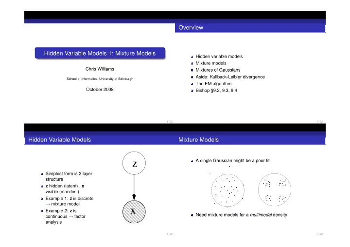
Hidden Variable Models

Simplest form is 2 layer structure z hidden (latent) , x visible (manifest) Example 1: z is discrete → mixture model Example 2: z is continuous → factor analysis

z

• x

3 / 22

Mixture Models

A single Gaussian might be a poor fit

x

. . . . . . .. . . . . . . . . . . . . . . . . . . . . . . .. ... . . . .... . . . .... . . . . . . ... ... . . . . . .

Need mixture models for a multimodal density

4 / 22

Let z be a 1-of-k indicator variable, with

j zj = 1.

p(zj = 1) = πj is the probability of that the jth component is active 0 ≤ πj ≤ 1 for all j, and k

j=1 πj = 1

The πj’s are called the mixing proportions p(x) =

k

• j=1

p(zj = 1)p(x|zj = 1) =

k

• j=1

πjp(x|θj) The p(x|θj)’s are called the mixture components

5 / 22

Generating data from a mixture distribution

for each datapoint Choose a component with probability πj Generate a sample from the chosen component density end for

6 / 22

Responsibilities

γ(zj) ≡ p(zj = 1|x) = p(zj = 1) p(x|zj = 1)

• ℓ p(zℓ = 1) p(x|zℓ = 1)

= πj p(x|zj = 1)

• ℓ πℓ p(x|zℓ = 1)

γ(zj) is the posterior probability (or responsibility) for component j to have generated datapoint x

7 / 22

Maximum likelihood estimation for mixture models

L(θ) =

n

• i=1

ln   

k

• j=1

πjp(xi|θj)    ∂L ∂θj =

• i

πj

• ℓ πℓp(xi|θℓ)

∂p(xi|θj) ∂θj now use ∂p(xi|θj) ∂θj = p(xi|θj)∂ln p(xi|θj) ∂θj and therefore ∂L ∂θj =

• i

γ(zij)∂ln p(xi|θj) ∂θj

8 / 22

Example: 1-d Gaussian mixture

p(x|θj) = 1 (2πσ2

j )1/2 exp −

• (x − µj)2

2σ2

j

• ∂L

∂µj =

• i

γ(zij)(xi − µj) σ2

j

∂L ∂σ2

j

= 1 2

• i

γ(zij)

• (xi − µj)2

σ4

j

− 1 σ2

j

• 9 / 22

At a maximum, set derivatives = 0 ˆ µj = n

i=1 γ(zij)xi

n

i=1 γ(zij)

ˆ σ2

j =

n

i=1 γ(zij)(xi − ˆ

µj)2 n

i=1 γ(zij)

ˆ πj = 1 n

• i

γ(zij).

10 / 22

Generalize to multivariate case ˆ µj = n

i=1 γ(zij)xi

n

i=1 γ(zij)

ˆ Σj = n

i=1 γ(zij)(xi − ˆ

µj)(xi − ˆ µj)T n

i=1 γ(zij)

ˆ πj = 1 n

• i

γ(zij). What happens if a component becomes responsible for a single data point?

11 / 22

Example

2 4 6 −2 −1 1 2

Initial configuration Final configuration

2 4 6 −2 −1 1 2

Mixture p(x) Posteriors P(j|x)

100 200 1 2 0.2 0.4 0.6 0.8 1 Component 1: µ = (4.97,−0.10) σ2 = 0.60 prior = 0.40 Component 2: µ = (0.11,−0.15) σ2 = 0.46 prior = 0.60

(Tipping, 1999) 12 / 22

Example 2

−1 1 2 3 −1.5 −1 −0.5 0.5 1 1.5

Initial configuration Final configuration

−1 1 2 3 −1.5 −1 −0.5 0.5 1 1.5

Mixture p(x) Posteriors P(j|x)

100 200 1 2 0.2 0.4 0.6 0.8 1 Component 1: µ = (1.98,0.09) σ2 = 0.49 prior = 0.42 Component 2: µ = (0.15,0.01) σ2 = 0.51 prior = 0.58

(Tipping, 1999) 13 / 22

Kullback-Leibler divergence

Measuring the “distance” between two probability densities P(x) and Q(x). KL(P||Q) =

• i

P(xi) log P(xi) Q(xi) Also called the relative entropy Using log z ≤ z − 1, can show that KL(P||Q) ≥ 0 with equality when P = Q. Note that KL(P||Q) = KL(Q||P)

14 / 22

The EM algorithm

Q: How do we estimate parameters of a Gaussian mixture distribution? A: Use the re-estimation equations ˆ µj ← n

i=1 γ(zij)xi

n

i=1 γ(zij)

ˆ σ2

j ←

n

i=1 γ(zij)(xi − ˆ

µj)2 n

i=1 γ(zij)

ˆ πj ← 1 n

• i

γ(zij). This is intuitively reasonable, but the EM algorithm shows that these updates will converge to a local maximum of the likelihood

15 / 22

The EM algorithm

EM = Expectation-Maximization Applies where there is incomplete (or missing) data If this data were known a maximum likelihood solution would be relatively easy In a mixture model, the missing knowledge is which component generated a given data point Although EM can have slow convergence to the local maximum, it is usually relatively simple and easy to implement. For Gaussian mixtures it is the method of choice.

16 / 22

The nitty-gritty

L(θ) =

n

• i=1

ln p(xi|θ) Consider for just one xi first log p(xi|θ) = log p(xi, zi|θ) − log p(zi|xi, θ). Now introduce q(zi) and take expectations log p(xi|θ) =

• zi

q(zi) log p(xi, zi|θ) −

• zi

q(zi) log p(zi|xi, θ) =

• zi

q(zi) log p(xi, zi|θ) q(zi) −

• zi

q(zi) log p(zi|xi, θ) q(zi)

def

= Li(qi, θ) + KL(qi||pi)

17 / 22

From the non-negativity of the KL divergence, note that Li(qi, θ) ≤ log p(xi|θ) i.e. Li(qi, θ) is a lower bound on the log likelihood We now set q(zi) = p(zi|xi, θold) [E step]

Li(qi, θ) =

• zi

p(zi|xi, θold) log p(xi, zi|θ) −

• zi

p(zi|xi, θold) log p(zi|xi, θold)

def

=Qi(θ|θold) + H(qi)

Notice that H(qi) is independent of θ (as opposed to θold )

18 / 22

Now sum over cases i = 1, . . . , n L(q, θ) =

n

• i=1

Li(qi, θ) ≤

n

• i=1

log p(xi|θ) and L(q, θ) =

n

• i=1

Qi(θ|θold) +

n

• i=1

H(qi)

def

= Q(θ|θold) +

n

• i=1

H(qi) where Q is called the expected complete-data log likelihood. Thus to increase L(q, θ) wrt θ we need only increase Q(θ|θold) Best to choose [M step] θ = argmaxθQ(θ|θold)

19 / 22

θold θnew

L (q, θ) ln p(X|θ)

Chris Bishop, PRML 2006 20 / 22

EM algorithm: Summary

E-step Calculate Q(θ|θold) using the responsibilities p(zi|xi, θold) M-step Maximize Q(θ|θold) wrt θ EM algorithm for mixtures of Gaussians µnew

j

← n

i=1 p(j|xi, θold)xi

n

i=1 p(j|xi, θold)

(σ2

j )new ←

n

i=1 p(j|xi, θold)(xi − µnew j

)2 n

i=1 p(j|xi, θold)

πnew

j

← 1 n

n

• i=1

p(j|xi, θold).

[Do mixture of Gaussians demo here]

21 / 22

k-means clustering

initialize centres µ1, . . . , µk while (not terminated) for i = 1, . . . , n calculate |xi − µj|2 for all centres assign datapoint i to the closest centre end for recompute each µj as the mean of the datapoints assigned to it end while k-means algorithm is equivalent to the EM algorithm for spherical covariances σ2

j I in the limit σ2 j → 0 for all j

22 / 22