Z 1 = a 11 X 1 + a 12 X 2 + + a 1n X n Coefficients for linear - - PowerPoint PPT Presentation

Principal Components Analysis (PCA)

Multivariate Fundamentals: Rotation

Objective: Find linear combinations of the original variables X1, X2, …, Xn

to produce components Z1, Z2, …, Zn that are uncorrelated in order of their importance, and that describe the variation in the original data Components will decrease in the amount of variation they explain (i.e. the first component (Z1) will explain the greatest amount of variation, the second component (Z2) will explain the second greatest amount of variation, and so forth.

Karl Person (1857-1936) Herold Hotelling (1895-1974)

The math behind PCA

Z1 = a11X1 + a12X2 + … + a1nXn

First principal component (column vector) Column vectors of original variables

Principle components are the linear combinations of the original variables Principle component 1 is NOT a replacement for variable 1 – All variables are used to calculate each principal component For each component: The constraint that a11

2 + a12 2 + … + a1n 2 = 1 ensures Var(Z1) is as large as possible

Coefficients for linear model

The math behind PCA

• Z2 is calculated using the same formula and constraint on a2n values

However, there is an addition condition that Z1 and Z2 have zero correlation for the data

• The correlation condition continues for all successional principle components

i.e. Z3 is uncorrelated with both Z1 and Z2

• The number of principal components calculated will match the number of

predictor variable included in the analysis

• The amount of variation explained decreases with each successional principal

component

• Generally you base your inferences on the first two or three components

because they explain the most variation in your data

• Typically when you include a lot of predictor variables the last couple of

principal components explain very little (< 1%) of the variation in your data – not useful variables

PCA in R

PCA in R:

princomp(dataMatrix,cor=T/F) (stats package)

Define whether the PCs should be calculated using the correlation or covariance matrix (derived within the function from the data) You tend to use the covariance matrix when the variable scales are similar and the correlation matrix when variables are on different scales Default is to use the correlation matrix because it standardizes to data before it calculated the PCs, removing the effect of the different units Data matrix of predictor variables You will assign the results back to a class once the PCs have been calculated

PCA in R

PCA in R

Loadings – these are the correlations between the original predictor variables and the principal components Identifies which of the original variables are driving the principal component

Example:

Comp.1 – is negatively related to Murder, Assault, and Rape Comp.2 – is negatively related to UrbanPop

Eigenvectors

PCA in R

Scores – these are the calculated principal components Z1, Z2, …, Zn These are the values we plot to make inferences

PCA in R

Variance – summary of the output displays the variance explained by each principal component Identifies how much weight you should put in your principal components

Example:

Comp.1 – 62 % Comp.2 – 25% Comp.3 – 9% Comp.4 – 4 %

Eignenvalues divided by the number of PCs

PCA in R - Biplot

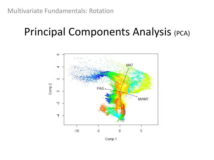
Data points considering Comp.1 and Comp.2 scores (displays row names) Direction of the arrows +/- indicate the trend of points (towards the arrow indicates more of the variable) If vector arrows are perpendicular then the variables are not correlated If you original variables do not have some level of correlation then PCA will NOT work for your analysis – i.e. You wont learn anything!